Williamson Simple model:

[As M = 0 in this model,  which is the constraint function.]
Because, M = 0, πR = π we have
ID = π - π0 - T and
substituting this in the utility function we get,

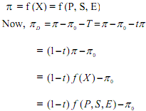
Assuming no lump-sum tax, T = tπ .
Therefore, the utility function becomes,

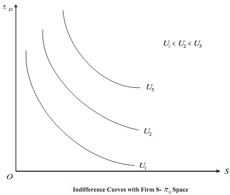
To arrive at the equilibrium, managerial indifference curves are drawn in the S - πD space. These curves indicate the combinations of , and π which yield the same level of utility to the managers. It is assumed that the ICs are downward sloping convex (representing diminishing MRS of S for πD ). It is further assumed that any of these curves does not intersect the axes. With these assumptions, we obtain the ICs as shown in the following Figure.

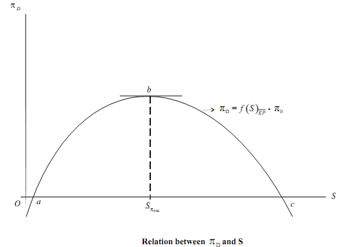
t is exogenously given from the tax laws and so is , π0 because it is the demand for dividends of shareholders. Also, considering that the market environment is given by E and assuming that output is chosen optimally according to MR = MC, the relation between D π and S is shown below in Figure.


At the initial stages of production and up to the level of output where profit is maximum, both πD and S increase. Beyond point b, (where π = maximum profit) if production increases, then profit starts declining although S increases. Beyond point c, the 0 = π , and the minimum profit constraint is not satisfied. Therefore, points to the left of a and to the right of c are not feasible. Superimposing Figure, we get Figure, where the equilibrium is determined by the point of tangency between the profit-staff curve and the highest possible managerial indifference curve, as represented point e in the figure.
Given that the managerial indifference curves are downward sloping, it follows that the equilibrium will be on the falling section of the profit-staff curve. This shows that the preference of managers for staff expenditures (S*) is greater than that of a profit-maximiser.
