Exponential Smoothing:

It is a refined moving average forecasting method in which past data is given weights in an exponential manner so that the most recent data carries greater weight in the moving average. This is of two kinds.

1. Simple Exponential Smoothing, and

2. Adjusted Exponential Smoothing.

Simple Exponential Smoothing

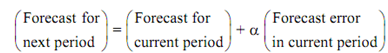
The forecast for the next period is computed as equal to forecast for the current period plus a fraction of the forecast error in the current period.

F_{t + 1} = F_t + α (D_t - F_t)     . . . (1)

where  F_{t + 1} = forecast for the next period,

F_t = forecast for the current period,

D_t = actual demand for the current period, and

α = smoothing constant, 0 < α < 1.

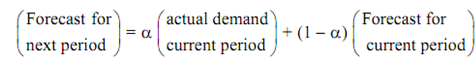
We may write down Eq. (1) in the following  way

F_{t + 1} = α D_t + (1 - α) F_t

= α D_t + α (1 - α) D_{t - 1} + α (1 - α)² D_{t - 2} + . . . + α (1 - α)^{t - 1} D₁ + α (1 - d)ⁿ D_{t - n}

It shows that forecast of demand for the next period is a weighted moving average of previous demand data with the weights decreasing exponentially with the age of the data. Although the name of the technique. While α is low, more weight is given to past data, and when it is high, more weight is given to the recent data. The effect of different values of α is shown in the following table.

Table: Magnitudes of Exponential Smoothing Coefficients for two Values of α

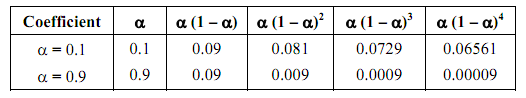
This is interesting to note that when α = 0.9, then 99.99 percent of the forecast value is find out by the four most recent demands however while α is as low as 0.1, only 34.39 percent of the average is due to these last four periods. For the value of α as high as 1, each forecast would reflect a total adjustment to the recent demand and the forecast would simply be the last period's actual demand.

The demand fluctuations being typically random and sporadic, in general the value of α are decided in the range 0.005 to 0.3 in order to smooth the forecast. The exact value of α to be employed for attaining satisfactory forecast is usually determined by trial-and-error testing of different smoothing constants to discover the one that has a good fit with past data. Alternatively, this is not a bad idea to start with a value of α as 0.2 or 0.3 and watch the performance for a few months.

Whenever a seasonal pattern is known to exist, it can be desirable to make the seasonal adjustment to the exponentially smoothed forecast, just as with a time series. The procedure can be simply stated in three steps.

Step 1 : Deseasonalize the actual demand

Step 2 : Compute a deseasonalized forecast

Step 3 : Adjust the forecast by multiplying with the seasonal index.