We  have mentioned  earlier that  in  simultaneous models the explanatory variables and the error terms are not independent. So one of the important assumptions of OLS that there should be  no  covariance between  the explanatory variable and  the  error term is violated. As a consequence the estimators are not consistent.

In  order to  show  that the  parameters  are  not  conbistent,  let  us  take  a  concrete example. Let us  go  back  to  the simple Keynesian model  of  income determination given  in  Example.  Suppose  we  want  to estimate the parameters  of  the consumption function  given  at eq. without taking into "account the  income identity. As you know, the standard assumptions under OLS.

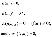
In  the case of the consumption function we will first show that  Y_t and  u_t are correlated and then prove that OLS estimate is  an  inconsistent estimator of P,.

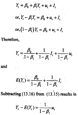
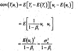
Since σ²  is positiveby  defmition, the aovariance between  Y  and  u  given in is  bound  to  be  different  fiom  zero. Let  us  look  back  to  eq i.e.,

C_i = β₀+ β₁Y_t+ u_t . Here, the explanatory variable  Y,  and  the error term  u,  are correlated, which violates the  assumption of the clissical linear regression model that the  disturbaces  are  independent  or  at  least  uncorrelated  with  the  explanatory variables. As noted  previously, the OLS  estimators in  this situation are inconsistent.

To show that she OLS estimator .is'  dnsistent because of correlation between  Y_t and u_t  , we ptoceed  as follows:

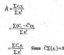
We  know  that the  sum of the deviations ftom arithmetic mean is zero. Therefore, ∑Y_t = 0.

Let us substitute in equation 4 for C_t . Thus we obtain

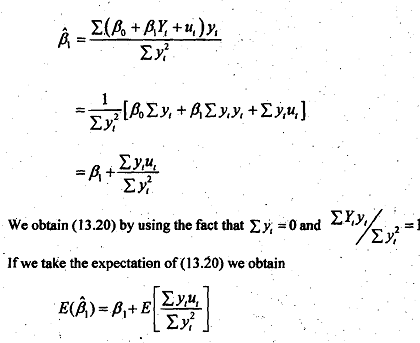
As expectation operator is a  iinear operator, we cannot evaluate . since But  intuitively  it  is clear that β₁, will  be unbiased  only if . Though we have shown in that the covariance  between Y and u is nonzero that does not mean cov  (y_tu_t )  ≠ 0, since cov (y_iu_i) is a population concept. It is not exactly equal to ∑y_tu_t  which  is a sample measure,  aIthough aq the sampk size  increases indefinitely the latter will tend toward the fmmer,  But if the sample size increases  indefinitely, then we can resort  to  the  concept of consist estimator and  thus  find  out what happens  to β₁, as n,  the smpIe size, increase indefinitely.  In  short  when we cannot explicitly evaluate the expected value of an estimator, as in,  we can turn our attention  to its behavior in the  sample.

Now  an estimator is said to be consistent if  its probablity limit,  of plim  for short, is equal to its tnrt  (population) value. Therefore, to tow that  P, of  is inconsitennt:  we must show that its plim  is not equal to the true β₁.

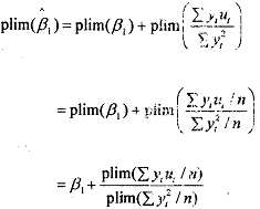
Where in  the second step we have divided  by  the total number of observations in  the  sample n so that the quantities  in  the parentheses are now  the sample covariance  between Y  and  u and the sample variance of Y ,  respective. In  other words, states that the probability  limit (plirn) of  β₁ is equal to true β₁ plus the ratio of the plim of the sample covarance  between  Y and  u to the plim of the  sample variance of  Y. Now as  sample  size n increases indefinitely, one would  expect  the sample covarince  between  Y  and  u  to  approximate the  true population covariance E[Y_t - E(y_t)] [u_t - E(u_t)] which from is equal  to

Similarly, as  n  tends to infinity, the sample variance of  Y  will  approximate its 2 population variance, say σ_y² . Therefore, equation may be written as

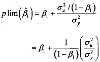
Given  that  O<β₁ <.l  and  that  σ²  and  σ_y² are  both  positive,  it  is obvious  from equation that  plim  (β₁) will  always  be  greater  than β₁ that  is,  β₁ will overestimate the true paramete,  β₁  in other words, β₁ is a biased estimator,  and the bias will not disappear no matter how large the sample size.