Heat Rejection

To recognize why an efficiency of 73% is impossible we should analyze the Carnot cycle, then compare the by cycle using real and ideal machineries. We will do this by observing at the T-s diagrams of Carnot cycles by using both real and ideal machineries.

The energy added to a functioning fluid throughout the Carnot isothermal expansion is given by q_s. Not all of the energy is available for use by the heat engine as a part of it (q_r) should be discarded to the atmosphere. This is represented by:

q_r =T_o Δs in units of Btu/lbm,

Here:

 T_o is the average heat sink temperature of 520°R. The available energy (A.E.) for Carnot cycle might be represented as:

A.E. = q_s - q_r

Replacing the equation q_r =T_o Δs for q_r provides:

A.E. = q_s -T_o Δs in units of Btu/lbm.

and is equivalent to the region of the shaded area tagged available energy in the figure shown below among the temperatures 1962° and 520°R. From the figure shown below it can been seen that any cycle operating at a temperature of less than 1962°R will be less proficient. Note that by mounting materials capable of enduring the stresses above 1962°R, we could greatly add to the energy available for use via the plant cycle.

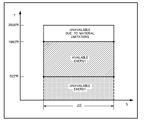
Figure: Carnot Cycle

From the equation q_r =T_o ?s, one can observe why the change in entropy can be stated as a measure of the energy unavailable to do work. When the temperature of the heat sink is acknowledged, then the change in entropy does correspond to a measure of the heat discarded by the engine.

The figure shown below is a usual power cycle used by a fossil fuel plant. The functioning fluid is water that places certain limitations on the cycle. When we wish to bound ourselves to operation at or beneath 2000 psia, it is eagerly apparent that constant heat addition at our utmost temperature of 1962°R is not possible (Figure below, 2' to 4). In reality, the nature of water and certain elements of the process controls need us to add heat in a constant pressure process rather (as shown in figure, 1-2-3-4). Since of this the average temperature at which we are adding heat is faraway below the maximum acceptable material temperature.

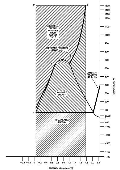
Figure: Carnot Cycle vs. Typical Power Cycle Available Energy

As we seen, the actual available energy (region under the 1-2-3-4 curve, above figure) is less than half of what is available from the ideal Carnot cycle (region under 1-2'-4 curve, Figure above) operating among the identical two temperatures. The usual thermal efficiencies for fossil plants are on the order of 40% whereas nuclear plants have efficiencies of the order of 31%. Note that such numbers are less than 1/2 of the maximum thermal efficiency of the ideal Carnot cycle computed.

The figure shown below illustrates a proposed Carnot steam cycle superimposed on a T-s diagram. As shown, it has many problems which make it undesirable as a practical power cycle. At first a great deal of pump work is needed to compress a two phase mixture of water and steam from point 1 to the saturated liquid state at point 2. Secondly, this similar isentropic compression will probably outcome in some pump cavitations in the feed system. Lastly, a condenser designed to generate a 2-phase mixture at the outlet (i.e., at point 1) would pose scientific problems.

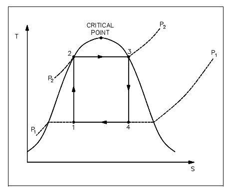
Figure: Ideal Carnot Cycle

Early thermodynamic developments were centered on improving the performance of contemporary steam engines. It was pleasing to construct a cycle which was as close to being reversible as possible and would better lend itself to the characteristics of steam and procedure control than the Carnot cycle did. Towards this last part, the Rankine cycle was build up.

The major feature of the Rankine cycle, shown in figure below, is that it limits the isentropic compression procedure to the liquid phase only (as shown in figure below points 1 to 2). This reduces the quantity of work needed to achieve operating pressures and ignores the mechanical troubles related with pumping a 2-phase mixture. The compression procedure shown in figure below among points 1 and 2 is greatly overstated. In reality, a temperature increase of only 1°F takes place in compressing water from 14.7 psig at a saturation temperature of 212°F to 1000 psig.

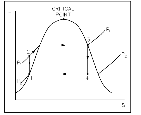
Figure: Rankine Cycle

In a Rankine cycle available and not available energy on a T-s diagram, similar to a T-s diagram of a Carnot cycle, is symbolized by the regions under the curves. The maximum the unavailable energy, the less proficient the cycle is.

From the T-s diagram (the figure is shown below) it can also be observe that when an ideal component, in this situation the turbine, is substituted with a non-ideal component, the efficiency of the cycle will be decreased. This is due to the fact that the non-ideal turbine invites a rise in entropy that raises the area under the T-s curve for the cycle. Though the rise in the region of available energy (3-2-3', figure shown below) is less than the rise in region for unavailable energy (a-3-3'-b, figure shown below).

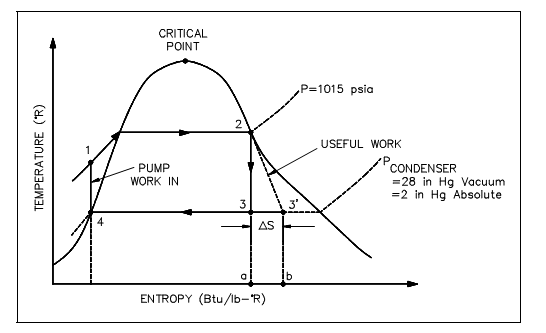
Figure: Rankine Cycle with Real versus Ideal

The similar loss of cycle efficiency can be observed whenever two Rankine cycles are compared (as shown in figure below). By using this kind of comparison, the quantity of discarded energy to available energy of one cycle can be compared to the other cycle to establish which cycle is the most proficient, that is. Has the least quantity of unavailable energy.

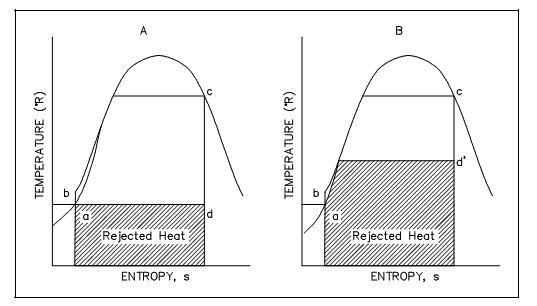
Figure: Rankine Cycle Efficiencies T-s

An h-s diagram can also be employed to compare systems and help to establish their efficiencies. Similar to the T-s diagram, the h-s diagram will illustrate (figure shown below) that replace non-ideal components in place of ideal components in a cycle, will outcome in the decrease in the cycles efficiency. This is since a change in enthalpy (h) always takes place whenever work is complete or heat is added or eliminated in an actual cycle (i.e., non-ideal). This deviation from an ideal constant enthalpy (i.e., vertical line on the diagram) permits the inefficiencies of the cycle to be simply seen on a h-s diagram.

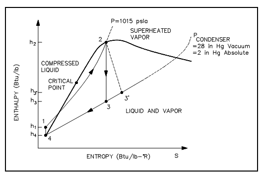
Figure: h-s Diagram