Operation of Insurance- State Contingent Commodities:

We have seen above that risk preference generates demand for insurance. Let us  now extend that discussion  by  taking insurance  as  a 'state contingent commodity'. That  is,  a good, which  you buy  now but only consume if a specific state of  the world arises. For example, when you buy  insurance you are buying a claim on Re. 1.00. Such insurance is purchased before the state of the world  is  known. You can only make  the  claim for  the  payout if the relevant state arises.

While analyzing consumer behaviour, we've drawn indifference maps across goods X,Y. Now we will draw indifference map across states of  the world: good, bad.

Consumers can use their endowment (equivalent to budget set) to shift wealth across states  of  the world via insurance, just like budget set can be  used  to shift consumption across goods, X, Y.  

Example

Two states of world, good and bad. Wealth in these two states and probability of occurrence of the states are given as, w_g = 120
w_b  =  40
Pr(g) = P = 0.75 and Pr(b) =  (1 -  P) = 0.25.

Then, E(w) = 0.75(120) + .25(40) = 100 and E(u(w)) <  u(E(w)) if agent is risk averse.

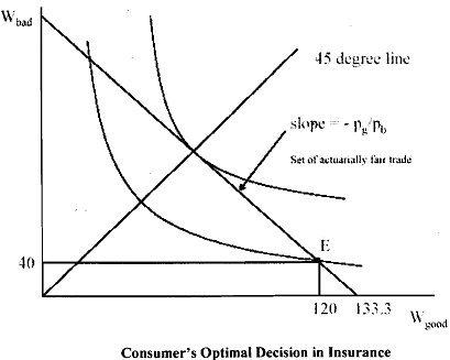
Let us look at Figure 20.5 to assess the consumer' optimal decision.

Let's say that this agent can buy actuarially fair insurance. If you want Re.l.OO  in Good state, this will sell of Rs.0.75  prior to the state being revealed.
If  you want Re.l .OO  in Bad  state, this will sell for Rs.0.25 prior  to  the  state being revealed. As  you  can observe  the  price  set  is such  that  these are  the  expected probabilities of making the claim. So, a risk neutral agent (say LIC  of  India) could sell you  insurance against bad states at a price of Rs.0.25 and insurance against good states (assuming you wanted to buy it) at a price of Rs.0.75. The price ratio is therefore

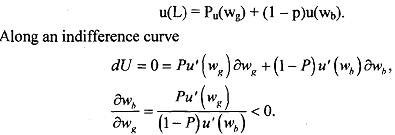
The set of fair trades among these states can be viewed as a budget set and the slope is . Now we bring in indifference curves. Recall that the utility of this lottery (the endowment) is:

Provided  that  u()  concave,  these  indifference curves are  bowed  towards the origin  in probability space. We  can  then  prove  that  indifference curves are convex to origin by taking second derivatives. But intuition is straightforward.

Flat  indifference curves  would indicate  risk neutrality  - because  for risk neutral agents, expected utility is linear in expected wealth.

Convex indifference curves means that you must be compensated to bear risk. Thus, if I gave you Rs.133.33 in good state and 0 in bad state, you are strictly worse off than getting Rs.  100 in each state, even though your expected wealth is

 E(w) = 0.75 .  133.33 + 0.25  .  0 = 100

So,  I  would  need to  give  you  more than  Rs.133.33 in  the  good  state  to compensate for this risk. It  is  easy to  see that there are potential  utility improvements from reducing risk.  In  the figure,  u,  +  u,  is the gain  from shedding risk. Also notice from Figure 20.5  that along the 45'  line, w,  = wb. But if w,  = wb,  this implies that

Hence, the  indifference curve will be  tangent  to the budget set at exactly the point where wealth  is  equated across states. This  is a very strong restriction that  is imposed by  the expectedutility property: The slope of the indifference curves in expected utility space must be tangent to the odds ratio.