Efficiencies of competitive equilibrium:

We now turns to three important efficiencies  generated by  the free market when on equilibrium, viz.,  (i) productive efficiency,  (ii) allocative efficiency and (iii) product-mix efficiency.

Productive (Technical) Efficiency

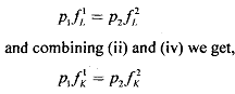
Productive efficiency  requires that we cannot produce more of a good without producing less of another. In order to appreciate its underlying idea, we may have  to  recall the  concept of opportunity cost. That  is, the cost of producing more X can be readily measured by  the reduction in Y output. Let us consider the marginal conditions described in  (i) - (iv). Combining (i) and (iii) we get,  

This means when we consider economic efficiency, marginal revenue product of  labor  (and capital) must be  the same in both  the industry. This mechanism is analogous to Smith invisible hand mechanism, which  says that  if the above two  relationships do not  hold,  there will  be  competitive bidding among the employers  in  the  concerned industries  such  that  the equality will  again  be restored.

It  can be proved  that  A,  is the  imputed value of  labor and  A,  is the  imputed value of  capital. Thus, we can  use above two Lagrange multipliers as proxy for wages and rent respectively. Then, from (i) and  (ii), we get

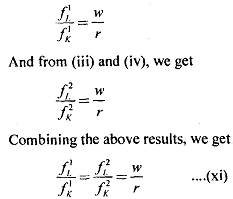
that is, the sector equates  the ratios of marginal productivities cf factors  to the price ratio and  these ratios are equated across sectors. Consequently, we  can say that productive (technical)  efficiency is satisfied in the equilibrium. We can explain the above result using the Edgeworth Box diagram.

Figure shows the set of factor allocations in  production for which Pareto efficiency is achieved. (By Pareto efficiency we mean  no  further gains from trade can be  obtained if one moves from  the above allocation.  i.e.,  there is no mutually possible betterment if one move from a Pareto efficient allocation).

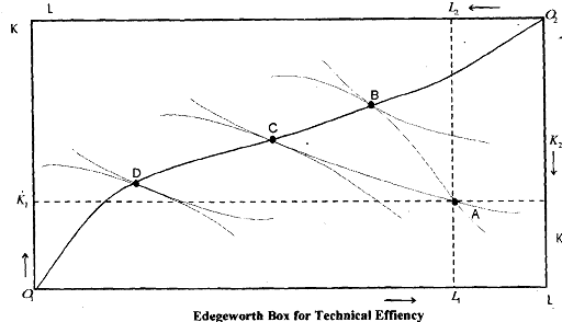
The X-axis and Y-axis of the box  are total  endowment of  labor and capital respectively. Labor  is plotted horizontally and capital vertically. With respect to  the origin O₁  we  have drawn  the isoquants for the  first  industry and with respect to the origin O₂  we have drawn isoquants for the second industry. The  efticient  factor  allocation  consists of the points are those  input combinations  for  which  slopes of  the isoquants  for the  two industries are equal. This condition is given by  the equation (xi).
The curve O₁ O₂  is known as the efficiency locus or the contract curve, which is obtained by joining  the points at which  isoquants are tangent to each other.

Any  point, which is off the curve,  is  inefficient in  Pareto sense. For example consider the  initial  endowment point A. Movement form A  to points B or C (both of which  are on  the contract curve will  lead to  increase in  output for at least one industry while the output of the other industry will remain constant. Thus, there is  scope for mutual  betterment  if  the  allocation  point  is off  the contract curve. At all points on the contract curve, all possible gains fiom trade are exhausted. The efficiency  locus will  be  obtained through the  above invisible hand  (i.e., bargaining) mechanism  if there is no transaction cost involved  in  the process of bidding. It  is to be  noted  that every point on  the contract curve corresponds to a point on the production possibility frontier. Thus, the production possibility'frontier is one to one mapping of the contract curve from the  input space to the output space.