Normal Distribution

Normal distribution is perhaps the most widely used distribution in Statistics and related subjects. It has found applications in inquiries concerning heights and weights of people, IQ scores, errors in measurement, rainfall studies and so on. The probability density function p(x) of a continuous random variable that follows the normal distribution is given by

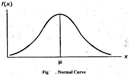
The normal density function is completely determined by the parameters μ and σ. It means that given the values of μ and σ, we can trace out the normal curve by obtaining the values of p(x) for different value of x. In fact, it can be shown that μ and σ are respectively the mean and the standard deviation of the normal distribution. When a random variable X follows normal distribution with mean μ and standard deviation σ we write it in symbols as X - N(μ, σ) and read as X follows normal distribution with meanp and standard deviation σ.' The normal curve is a symmetrical bell-shaped curve as shown in Fig.

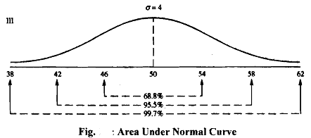
The normal curve stretches from - ∞ to + ∞. It is symmetric about its mean. The following area properties hold for a normal distribution. In Fig. 1.2 below we plot a normal curve with mean μ = 50 and standard deviation σ= 4.

a) 68.8 % of the area under the normal curve lies between the ordinates at μ - σ and  μ + σ. Thus in Fig,68.8% area is covered when x ranges between 46 and 54.

b) 95.5% of the area under the normal curve lies between the ordinates at ' μ-2σ and μ+2σ. In Fig. 1 95.5% are discovered when 42 ≤ X ≤ 58. 

c) 99.7% of the area (i.e., almost the whole of the distribution) under the normal curve lies between the ordinates at ,

μ - 3σ and ,μ + 3σ. In Fig. we find that 99.7% area is covered when 38 ≤ X ≤ 62.
A problem encountered here is that μ and  σ can take any value and finding out corresponding probability is time consuming. This problem is tackled by subtracting p from the normal variable and dividing it by σ. This way we '-', which has mean = 0 and obtain the 'standard normal variate', z = which has mean = 0 standard deviation = 1.

The probability density function of the standard normal variate, z, is given by

Once we obtain a standard normal variate, our seemingly hopeless task of obtaining probability areas for different combinations of ,μ and σ becomes elegantly simple. We should note that a standard normal variate has a unique mean of 0 and a unique standard deviation of 1. It means, if we can construct a table for probability areas of such a unique standard normal variate, it can be used for obtaining probability for any normal variable with any combination of mean and standard deviation. The only thing is that the given normal variable is to be transformed into the standard normal variate. In fact, such a table for areas (or probability) has been compiled for a standard normal variate.