Model of the Dominant Firm:

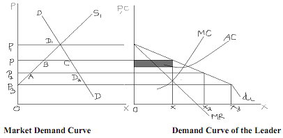
In this case, it is assumed that there is a large dominant firm, which has a considerable share of the total market, and some smaller firms each having a small market share. It is assumed also that the dominant leader knows the MC curves of the smaller firms. The leader adds these curves horizontally to arrive at the total supply by the small firms at each price. Or, we can think of the leader at best to have a fair idea from the past as to how much the small firms can sell at every price level. With this knowledge, the leader can obtain her own demand curve. This is illustrated in Figures below.

At each price, the demand for leader is the difference between total demand D at that price and total supply S₁. Accordingly, we can derive dL.  The profit maximising output level is determined by setting MR = MC, whereby output is Ox and price is OP. The other small firms would also sell at P, following the leader, and selling output, which does not maximise profit. There has to be some kind of an agreement among the firms regarding the market share, else the followers may not sell the amount required to maintain the profit maximising level of price.  

At price OP, PB gives the small firms supply and BC the leader's supply. At price OP3, AD2 gives the leader's supply.

Mathematical Representation 

In this model, the dominant firm knows the MC curves of the small firms. By adding these curves horizontally, it obtains the supply curve S₁ of the small firms as a function of price. Let us assume that S = 0.2P The dominant firm knows the market demand D = 50 - 0.3P

The dominant firm derives its own demand curve at any price as the difference (say X)  

i.e., X = D - S = 50 - 0.3P - 0.2P = 50 - 0.1P
or, P = 100 - 2X

Let the cost function of the dominant firm be C = 2X

Thus, profit function of the dominant firm is given by,

Δ = PX - 2X = (100 - 2X)X - 2X = 98X - 2X²
 
Differentiating partially with respect to X and setting the derivatives equal to zero we get,

∂Δ /∂X = 98 - 4X = 0, 

or, X = 24.5

The leader will set the price P = 100 - 2X = 100 - 2(24.5) = 51 and this will be the equilibrium price in the market.

The total quantity demanded in the market will be D = 50 - 0.3P = 34.7

This total demand is covered in the market with the leader producing X = 24.5 units and the small firms producing S = 0.2P = 0.2(51) = 10.2 units.