Cournot Model of Duopoly:

The model by Augustin Cournot deals with two profit maximising firms. Let the two firms be A and B. 

Assumptions

1) Each of the firms faces a linear market demand curve

2) Both sell identical products. In Counot's model, the two are assumed to sell mineral water.

3) The cost functions are identical and the marginal cost (MC) of each firm is zero.

4) Each firm assumes that the other would continue to produce the same output as in the last period.  

Diagrammatic Representation

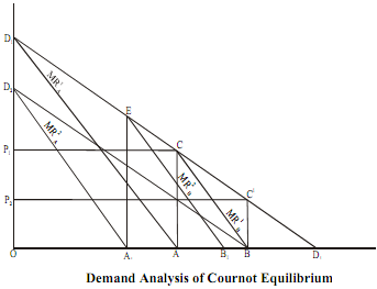
To arrive at the Cournot solution, let us assume that firm A is the first to produce and sell in the market. Let D₁D₁ be the linear market demand curve, as shown in Figure.The marginal cost =0 for both the firms. In the figure, this corresponds to the horizontal axis. Firm A being a profit maximiser, equates MR with MC and arrives at the output level OA (= ½ OD₁) and price OP₁ Suppose now firm B enters the market. As firm A is already selling OA amount of output, firm B would cater to OD₁ minus OA amount of the market demand, assuming that firm A will continue producing OA. Therefore, the portion of the market demand relevant to firm B is CD₁.This is so because B cannot sell anything at a price higher than OP1, as firm A is already present in the market and they are selling the same product. Hence the only other option open to firm B is to sell at a price lower than OP₁, whereby the market demand curve for B shrinks to CD₁. Firm B being a profit maximiser, produces output AB (= ½ A D₁) where MRB = MC = 0.

The output level supplied in the market after firm B's entrance is OA + AB(= ½ OD₁ + ¼ OD₁) = ¾ OD₁. As the output level goes up, the price in the market goes down to, say OP2. Next, firm A assumes firm B to continue producing AB and therefore the market demand that A can cater to is OD1 minus AB. In the diagram the market demand curve relevant to A is D2 B.  Once again setting MRA= MC = 0, firm A will produce OA₁ (= ½ OB= ½ * ¾ OD1 =3/8 OD1). Firm B now is assuming that firm A will continue producing OA1 and has ED1 as the relevant market demand curve. Setting MRB  = MC =  0 firm B would produce A1B1 = ½ A1 D₁ = ½ *(1- 3/8 ) OD₁  = 5/16 OD1. The total supply in the market would be OA₁ + A₁B₁= 3/8 OD₁ + 5/16 OD1 11/16 OD₁. As the market supply goes up the price comes down to say, OP₃.  Thus, we see that the output of firm A goes down whereas that of firm B goes up. This process continues until each one of the firms produces 1/3 OD₁.To see how, we derive the equilibrium output levels of each firm in the following. Let the total market demand be x units of output.

Let the total market demand be x units of output.

Output levels of firm A:

Period 1: x/2
Period 2: ½(1-1/4) x = 3x/8 = x/2 - x/8
Period 3: ½(1- 5/16) x = 11x/32 = x/2 - x/8 - x/32
Period 4: ½(1 - 21/64) x = 43x/128 = x/2 - x/8 - x/32 -x/128
In the nth period, the output of firm A is
 = x/2 - x/8 - x/32 -x/128 - .......
=  x/2 - [1/8 + 1/8 * (¼) + 1/8*(1/4)2 + ......... ] * x
=  x/2 -1/8 * [ 1/(1- 1/4)]*x   
= x/3
Output levels of firm B:
Period 2: ½(1/2)x = x/4
Period 3: ½(1- 3/8)x = 5x/16 = x/4 + x/16
Period 4: ½(1 - 11/32) x = 21x/64 = x/4 + x/16 + x/64
Period 5: ½(1 - 43/128) x = 85x/256 = x/4 + x/16 + x/64+x/256

In the n^th period, the output of firm B is

= x/4 + x/16 + x/64+x/256 +...
= [(¼)/1- ¼] * x  
= x/3