Stagnation Avoidance

It represents the situation while all ants construct the similar solution and thus the probability of searching newer path as zero. This kind of situation occurs mainly because of inappropriate tuning of the control parameter ρ or trail persistence. The stagnation may happen whereas its low quantity restricts the information flow, if the quantity ρ is extremely high. By generating a random number 'μ', this undesirable condition can be overcome, that is to be compared along with the intensity of pheromone trail τ_ij. For low amount of pheromone trail the possibility of occurrence of the event μ > τ_ij will be on upper side hence the newer path can be explored. Algorithm will stick on the particular edge, if pheromone trail is extremely high. Hence, the system is prevented from stagnating at a specific point. The modifications discussed on top that have been incorporated in the common ACO algorithm and the flowchart of the similar is represents in following figure.

Definition

Specified a set of part types P = {P₁, P₂ ... P_|P|} associated along with the set of alternative

|P| process plans P_i  = {Pi₁ , Pi₂ ... Pi^|Pi|} , processing times

 P_r Ti^j = {Pr Ti₁ , Pr Ti₂  ... Pr_i ^|Pri|} and number of steps S_i  = {Si₁ , Si₂  ... Si^|Pi| }

Here, i ∈ 1, 2 . . . | P |) such that the processing is to be carried over the resources as machines, tools,  fixtures whose availability is being indicated by the corresponding ones in the binary incidence matrix I, the problem is to choose a plan as a node in graphical representation p ∈ Pi for the processing of all parts type i or  i^th cluster of nodes such that the total processing cost is minimized subject to the constraint such only one node is to be chosen from all clusters.

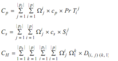
For the above definition, the cost function or C is described as the weighted sum of overall cost associated along with the processing time or C_P, number of steps comprised or C_S and the hamming distance or C_H signifying the dissimilarity between the process plans that is the problem is:

Minimize

                                       C = A × (C_p  + C_s ) + B × C_H ....................Eq(6)

Such as:

Here, A and B are the constants; Ωⁱ_j is binary decision variable which considered as the value 1 if the plan j is chosen for processing of part i; C_P is the cost per unit time; C_S indicate the cost per step; and D (i, j)(k, l) is the hamming distance among plan j or of part i and plan l or of part k that shows the dissimilarity count of the two plans computed by using incidence matrix I.

I is a binary matrix.

 And λ = total number of machines, tools and fixtures = M + T + F along with each 1 as per to the requirement of particular alternative for a plan.

Table no.3: Problem Characteristics for demonstration

Hamming distance or C_H is explained as weighted sum of number of resources unlike in two plans i or part j and k or part l; so mathematically:

Here, w_m, w_f and w_t are weight factors corresponding to the tools, fixtures and the machine as;  Δ^m_k and Δ^t_k, Δ^f_k are the binary decision variables that consider as the value 1 while the  k∈ tool, fixture or machine and corresponding values in incidence matrix are not similar. In the underlying problem, five parts have been considered with a total of twelve plans. Other parameter values concerned to the problem definition are given in Table no.3

Initialize the pheromone trails for each edge by an amount ε.

Initialize the visibility of each plan node l (part k) from a plan node j (part i), J_i,j as given below as:

Initialize some parameters as like n, α and β, iter.maximum

Input the process plans and compute the relevant data concerned to problem such is hamming distance matrix D_H for problem type 1 and D_S, SI and μ for problem type 2.

Set iter.current = 0.

Begin

Begin for each ant

Randomly place the ant on a node

Enter the selected node in Tabu1

Update Tabu2

Begin

Generate a random number u (0 ≤ u ≤ 1)

Create Tabu2 (excluding the nodes from the cluster of selected part types)

If u ≤ u0

Compute the probability for each probable node

Generate a random number s (0 ≤ s ≤ 1)

If s ≤ ξ^k_i,j (that is probability of j^th process plane of i^th part for ant k)

Choose the node with highest probability

Update Tabu1

Else

Else

 Select the next node randomly and Update Tabu1

 End

End

 Select the next node randomly and Update Tabu1

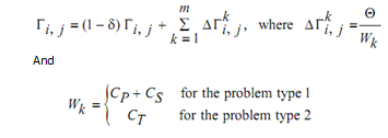
 Update best ant Update best global ant Update pheromone matrix like:

If (iter.corrent < iter.maximum) then continue begin

Else End

             Output best global ant

Programme no.2: Application of Ant Colony Optimization to PPS Problem