Pooling Equilibrium:
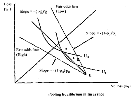
In a pooling equilibrium, both high and low risk types buy the same policy. That is, the insurer could offer a policy whose premium is based on the average probability of loss.
The equilibrium construct requires that this policy lie on the aggregate fair odds line. This implies that the policy earns neither negative nor positive profits. To arrive at the equilibrium, let us define il as the proportion of the high-risk population such that the expected share of the population experiencing a loss is given as

On the other hand, the expected share experiencing no loss is given as

If we look at the aggregate fair odds line's slope from Figure, it is given by

Notice that in the 'pooling' policy, A must lie on the aggregate fair odds line. For, if it is above, that would be unprofitable. Therefore, we would not have it in equilibrium. If it is below, there would be positive profits. That means, we cannot have it in equilibrium.
You may note that the figure is drawn with  It is important for the analysis. To appreciate the underlying reason, define


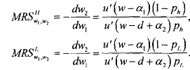
From the vNM property, we know the following:

Since both types, High and Low, agents are otherwise identical, we can write uh(w) = u1(w). This implies that

Thus, the slope of the indifference curve for type H is less steep than for type L. We know that the probability of loss is lower for type L. Therefore, type L must get strictly more income than H in the loss state to compensate for income taken from the no loss state. From this observation you can say that L types have steeper indifference curves for transfers of income between loss and no-loss states.
As seen above, the pooling equilibrium involves a cross-subsidy from L to H types, i.e., L types pay more than their expected cost and H types pay less than their expected cost. While both H, L types pay the same premium, H makes more claims which is met through cross subsidisation. Herein lies the problem for sustenance of the equilibrium which we see below.