Less than Perfect Multieollinearity Case:
We now consider the more realistic case of what happens to the parameter estimates of the MLRM when there is high but not perfect multicollinearity. Let us continue with our earlier example where income and wealth determine consumption expenditure. The case of 'less than perfect' multicollinearity arises when wealth for each individual is not a multiple of the current income of the person concerned. Say you observe that for the first person wealth is 9.5 times his income, for the second person this is 10.75 times his income and so on, such that on the average wealth is ten times the income, but with small deviations for each person (observation) in the data. In terms of equation we can say that v is an independent random variable (not correlated with any of the explanatory variables) with mean zero and small variance (compared to λ), and takes the value of -0.5 for the first person and 0.75 for the second person and so on (λ = 10 in this example).
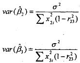
The bigger concern for the researcher arises fiom the impact of multicollinearity on the standard errors of the P estimates. Note that the estimates of the coefici&ts are as follows

where r23 is the correlation coefficient between X2 and X3. Therefore, it is obvious from the equations above that as the level of correlation between the two explanatory variables increases, i.e., the level of multicollinearity increases, or as r23 tends towards one, the variance estimates of the estimated coefficients var(β), increases. In the limiting case of perfect multicollinearity of course r23= 1 and the variances are infinite.