Consequences of heteroscedasticity:

Heteroscedasticity has two important implications for estimation. The first is that the least squares estimators, while still being linear and unbiased (in  the case of  finite but differing variances), are no longer efficient. They no longer provide minimum variance estimators among the class of linear unbiased estimators (that is, they are not BLUE). The  second  implicationls  that  the estimated variance  of  the least squares estimates  is biased; so  the usual tests of statistical significance, such as  t and Ftests are no  ionger valid. It  is thus important to test for and remove heteroscedasticity from the data.

Let us discuss  how  the changing  variance affects  the desirable  properties of  regression coefficients. We will consider two aspects: unbiasedness and minimum variance of the OLS estimate of P. Let the model in deviation form be

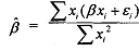
Then the least squares estimator of B,  is

By substituting the value of  y, from (1) in the above equation (2) we obtsin

By rearranging terms in the above we have

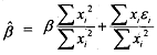
Under the standard assumption  of E(E) =  0 ,  we find that

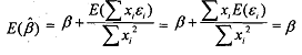
Notice that variances of the error terms play no role in  the proof that least-squares estimators are unbiased and consistent. Thus Pis  unbiased even  in the presence of heteroscedasticity.

The problem lies with  the variance  of  the estimated parameters p .  The variance of b under the assumption of homoscedasticity, is

When  there is heteroscedasticity  the variance of p  is quite  different fiom  (8.4). Let us derive the variance of b again.

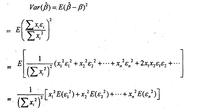
The variance of ci  is not constant in the presence of heteroscedasticits Suppose that 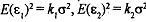and  so on. In general  terms we say  that E(ε_i)² =  kσ²,By using  the above in (8.5) we find that

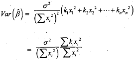
The difference between  (8.4) and (8.6) is the  factor.  If  kt and x, are positively correlated and then the classical least-squares estimation for the variance of ij will be overestimated. Thus  the variance is different from that when the disturbance was homoscedastic. It means that the least squares estimates are not efficient (that  is, not BLUE). It can
also  be shown  that  the OLS estimates  are not asymptotically  efficient  and  therefore, the tests of significance and confidence  limits do not apply.

Heteroscedastic  disturbance,  therefore, gives us false results whose significance is not liable to test. Hence, before testing for a hypothesis, the homoscedasticity of the disturbance term should be detected.