Integral of the velocity:

Equation 16 is also the value of the integral of the velocity, v, with respect to time, t, between the limits t_A  -t_B  for the case plotted in Figure.

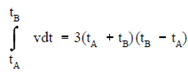
The cross-hatched area in Figure is the area under the velocity curve among t = t_A  and t = t_B.  The value of this area can be computed through adding the area of the rectangle whose sides are t_B  - t_A  and the velocity at t_A, that equals 6t_A  - t_B, and the area of the triangle whose base is t_B  - t_A  and whose height is the difference among the velocity at t_B  and the velocity at t_A, which equals 6t_B  - t_A.

Area = [(t_B  - t_A)(6t_A)] + [1/2(t_B - t_A) (6t_B -6t_A)]

Area = 6t_At_B - 6t²_A + 3t²_B -6t_At_B +3t²_A

Area = 3t²_B -3t²_A

Area = 3(t_B +t_A)(t_B -t_A)

This is accurately equal to the value of the integral of the velocity along with respect to time among the limits t_A and t_B.  Because the distance traveled equals the integral of the velocity with respect to time, ? vdt, and because this integral equals the area under the curve of velocity versus time, the distance traveled can be visualized as the area under the curve of velocity versus time.

For the case display in above figure, the velocity is increasing at a constant rate.  While the plot of a  function  is  not  a  straight  line,  the  area  under  the  curve  is  more  hard  to  determine. Therefore, it can be display that the integral of a function equals the area among the x-axis and the graphical plot of the function.

F(x)dx = Area between f(x) and x axis from x₁ to x₂

The mathematics of dynamic systems includes several different operations along with the integral of functions. As with derivatives, by practice, the integral of functions are not determined through plotting the functions and measuring the area under the curves.  While this approach could be used, methods have been developed that allow integral of functions to be determined directly based on the form of the functions.  In fact, the technique for taking an integral is the reverse of taking a derivative.  For instance, the derivative of the function f (x ) = ax + c, where a and c are constants, is a.  The integral of the function f (x ) = a, where a is a constant, is ax + c, where a and c are constants.

f (x ) = a

? f(x)dx  = ax +c

The integral of the function f (x) = ax n, where a and n are constants, is (a/n+1)x ⁿ⁺¹ +c is another constant.

 F(x) = axⁿ

∫ f(x)dx = a/n+1 xⁿ⁺¹ +c

The integral of the function f (x) = ae^bx, where a and b are constants and e is the base of natural logarithms, is  ae^bx/ b +c where c is another constant.

f (x ) = ae^bx

∫ f(x)dx = a/b e^bx + c

As with the methods  for searching  the derivatives  of functions, these  common  techniques  for searching the integral of functions are primarily  significant  only to those  who perform detailed mathematical  calculations for dynamic systems. These techniques are not encountered in the day-to-day operation of a nuclear facility. Therefore, it is worthwhile to understand that taking an integral is the reverse of taking a derivative. It is significant to understand what integral and derivatives are in terms of summations & areas under graphical plot, rates of change, and slopes of graphical plots.