Comparative Study between Cauchy Distribution Function and Boltzmann Distribution Function

Boltzmann Distribution

                                                      e^-(DME/T(b))

Cauchy Distribution

                                               T(b)/(T²(b) + (DME)²)

Here, ?ME = energy function, and T (β) = temperature.

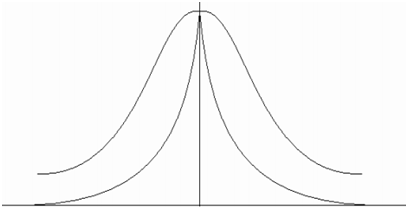
In following figure depicts the comparison between Boltzmann and Cauchy distribution. The wing of Cauchy distribution function has reached the deeper value however, the Boltzmann distribution has negligible value and hence less chance to flee from local minima. By employing Cauchy distribution we can pre-serve a local search and an occasional long jump to speed-up the organism state generation at T temperature.

           Figure: Comparison between Cauchy Distribution and Boltzmann Distribution Function

A lot of parallel algorithms have been proposed to overcome large computation time considered by serial simulated annealing or SA. In parallel simulated annealing the set of moves and computations completed in parallel should have serialization property; or else this adversely affects the convergence process. Parallel simulated annealing follows a single markov chain and performs multiple moves to decide the best choice at the higher temperature.

In order to decrees the computational time and to extend simulated annealing or SA over an array of samplers Thompson and Bilbro have planned for the sample-sort simulated annealing or SSA algorithm. Sample-sort simulated annealing algorithm consists of multiple or m samplers, and each sampler propagates simultaneously parallel to each other in search of the optimal resolution. The virtue of sample-sort simulated annealing algorithm lies in its serialization and parallelism properties that enable the algorithm to reject and accept the moves at lower and higher temperatures respectively. Inclusion of these two properties makes the sample-sort simulated annealing algorithm robust against the temperature variation.

All the m samplers are capable to exchange a less cost solution along with their neighbors however, does it probabilistically. In a row, they are lined up and exchange solutions along with samplers such are one or more moves away. The number of hope is named as the neighborhood. It adjusts Also the possibility of accepting a higher cost solution dependent upon the temperature of the neighboring samplers. Of course, serialization is maintained by adjusting the possibility of accepting a higher cost solution dependent upon the temperature. Thus, the objective of serialization is maintained in an easier mode or way than the earlier proposed simultaneously periodically interacting parallel annealing algorithms.

All of the m samplers operates at statistically monotonically raising temperature T_k, here k = 1, 2, . . . , m. Sample sort interacts along with their neighboring samplers N hopes away. All samplers tests and updates its position double in each generation; first along with the state of neighboring sampler as determined by the parameter N, then with a candidate solution generated uniformly in a neighborhood around its recent state. Bilbro and Thompson used possibility e₁ to accept the current state of sampler j, whereas for the second category of update; the acceptance possibility e₂ reduces to the common metropolis criteria.

                             e₁ (x_j¦x_i) = min {1,exp(-(f(x)_j - f(x)_i)){(1/T(x_i)) - (1/T(x_j))}} ...............

                              e₂ (x'¦x_i) = min {1,exp{-(f(x') - f(x_i)/T_i)}} ..................Eqn9