Coloured Stochastic PETRI NETS

In this section we discuss the modelling methodologies applicable to huge class of Flexible Manufacturing Systems or FMS that takes benefit of the differentiation among the Flexible Manufacturing Systems layout and the set of process plans consequent to various types of parts to be processed. Coloured Petri Nets or CPNs are the basis for the origin of the Stochastic Coloured Petri nets. Coloured Petri nets or CPNs are a high level Petri net or PN models that leads to compact net models by employing the idea of colours. Coloured Petri nets are more concise from the graphical viewpoint although have the similar modelling explanation power of classical Petri nets. This is attained by merging analogous places or transitions in a model into a single place or transition and relates colours to places, transitions and tokens to differentiate between different members. Therefore a transition may fire along with respect to different colours. After a transition fires, tokens are uninvolved and added to consequent places in a normal manner except that a functional dependency is specified among the colours of the transition firing and the colours of the occupied tokens.

As an instance, we can connect a set of machines processing jobs of different part types along with a single place. Tokens of that set are given various colours along with each colour identifying an exact type of machine. It might be occasionally necessary to group up tokens along with two or more attributes. For instance, a colour can characterize a condition of any part in relative to machine. Hence, a colour set could be any subset of the Cartesian product of the fundamental colour sets that can prove convenient in modelling the physical object beneath consideration. We can explain a colour Petri net like mathematically and a quintuple we can show it as following:

A CPN is explained as (P, T, C, IN, OUT) here,

• P and T are the set of transitions and places as already discussed.
• C (p₁) and C (t_j) are sets of colours connected with the place (p_i) and transitions (t_j).

Hence, we have:

C (p_i ) = {a_i1, a_{i 2} , . . . ,a_iui     }and

 u_i = | C (p_i )|   ∀ i = 1, 2, . . . , n

 C (t_j) = {b_j1, b_j2 , ... ,    b_jvj  }and

 v_j  = | C (t_j ) | ∀    j = 1, 2, . . . , m

a)      IN (p,t ) : C ( p) × C (t ) → N  is an input function.

b)      OUT (p,t) : C ( p) × C (t ) → N  is an output function.

We let a finite coloured sets for explaining the coloured Petri nets.

In the representation, we show places via circles and transitions are depicted via vertical or horizontal bars.

Illustration.1

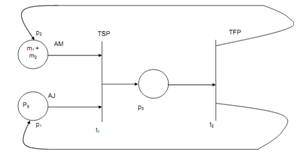
See a simple manufacturing system consisting of two machines M¹ and M² and processing two various types of parts.

All part type undergoes via a series of operation such can be either operated upon M₁ or M₂. While the processing of a part is finished then the part is unloaded from such system and a new part is loaded into it. The interpretation for transitions and places are specified in the Table no.1.

                                                     Table no.1: Interpretation of Places and Transitions of following figure.

The given figure portrays the Petri net model of the system.

                               Figure: Coloured Petri Net Model of Simple Automated and Manufacturing Systems

In the above Coloured Petri Net model, we include three colour sets: MACHS, PARTS and PARTS × MACHS where,

MACHS = {m₁, m₂},

PARTS = {J₁, J₂) additionally we have,

C (AJ) = {J₁, J₂}

C (AM) = m₁, m₂}

C (PROC) = MACHS × PARTS

And      C (TFP) = C (TSP) = MACHS × PARTS

We are here in a position to explain functions of input and output. First we seem an input function of the transition TSP along with reference to its different colours and colour J₁ of place AJ.

IN ( AJ , TSP) ( J₁ ), (m₁ , J₁ ) = 1

IN ( AJ , TSP) ( J₁ ), (m₁ , J ₂ ) = 0

IN ( AJ , TSP) ( J₁ ), (m₂ , J₁ ) = 1

IN ( AJ , TSP) ( J₁ ), (m₂ , J ₂ ) = 1

In the same way, regarding colour J₂ of the place AJ we have:

IN ( AJ , TSP) ( J₂ ), (m₁ , J₁ ) = 0

IN ( AJ , TSP) ( J₂ ), (m₁ , J₂ ) = 1

IN ( AJ , TSP) ( J₂ ), (m₂ , J₁ ) = 0

IN ( AJ , TSP) ( J₂ ), (m₂ , J₂) = 1

In normal IN (p₁, t₁) can also be represented as the |C(p₁)| × |C (t₁)| matrix.

IN ( p₁ , t₁ ) =

And we have IN (p₂, t₁) represented as |C(p₂)| × |C (t₁)|

IN ( p₂ , t₁ ) =