Training of an AFPN

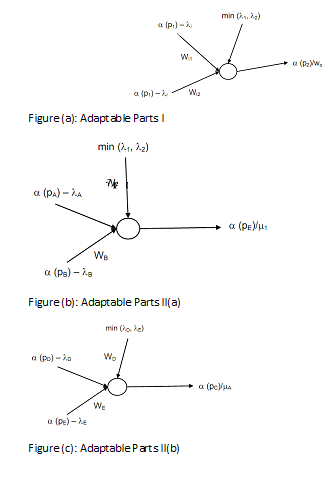
Before training an Adaptive Fuzzy Petri Nets, system inputs and outputs must be determined. Suppose that a system is described by weighted fuzzy production rule. Now, all the right hands of the rules are explained as the system outputs. If sufficient training data is available, the parameters can be adjusted well sufficient. As per to various types of system inputs, an Adaptive Fuzzy Petri Nets  is described into different types of sub-structures as represented in following figures (a) and (b) and (c). Hence a learning of an entire net can be decomposed into some simpler learning processes referring to these small subnets. Such fact greatly decreased the complexity of the learning algorithm.

                                                                 Figure (c): Adaptable Parts II(b)

Given weighted fuzzy production rule, this is assumed the threshold of each its antecedent propositions and its certainty factors are identified but the input weights W_I are not certain. In the conditions these weights are to be learned, where there are enabled transitions. On the other hand, for the type 1 fuzzy production rules, the input weights are 1, hence only type 2 and type 3 fuzzy production rules weights required to be learned. Moreover if we have a set of training data, via comparing the weights of the input arcs, this is simple to determine that transition is the dominating one at this place. Therefore training can be implemented whether enough data are available.

Example .2

{A, B, C, D, E, F, G} are the connected propositions of a knowledge-based system Γ. Among them exists the following rule as:

R1: If A and B Then E, λ_A, λ_B, w_A, w_B, (CF = μ₁)

R2: If C Then F, λ_C (CF = μ₂)

R3: If F Then G, λ_F (CF = μ₃)

R4: If D and E Then G, λ_D, λ_E, w_D, w_E (CF = μ₄)

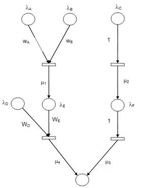
Based upon above translation principle such system is mapped into an Adaptive Fuzzy Petri Nets as shown in following figure.

                                                  Figure: A Representation of Knowledge Based System

In following real data is specified for this system as:

λ_A  = 0.5, λ_B  = 0.8, λ_C  = 0.3, λ_D  = 0.8, λ_E  = 0.1, λ_F = 0.4 and

 μ₁ = 0.8, μ₂  = 0.9, μ₃  = 0.6, μ₄  = 0.7 .

 As the required weights are not known, neural network technique is employed to learn these weights from actual data. While the set of inputs {α ( p_A ), α ( p_B ), α ( p_C ), α ( p_D )} are known, a human expert can give the consequent output ψ = {α ( pE ), α ( pF ), α ( pG )} .