Estimation and Inference:
Maximum Likelihood Estimation of the Probit and Logit Models:
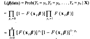
Both the prbbit and the logit models are non-linear models. Estimation of these models is usually based on the method of maximum likelihood. Each observation may be treated as a single draw from a Bernoulli distribution, with probability of success, (Y=1), equal to F(xiβ) and probability of failure, (Y=O), equal to [1 -F(xiβ)]. Under the standard sampling assumptions the observations are independent and we have the likelihood function,

where X = [x1, X2, x3, xn] is the matrix of data on the independent variables.

Taking the derivative with respect to βk, the elements of β, we have the first order conditions as

Here F, = F(xiβ), and$ is the probability density function given by (dFi/d (xiβ)). These equations are highly non-linear and solving them requires numerical optimization using iterative techniques such as the Newton-Raphson procedure. In the case of the probit model this is further complicated by the fact that the likelihood function has no closed form solution (is in the form of a definite integral) and must be evaluated numerically. In contrast the logit model is computationally more tractable.
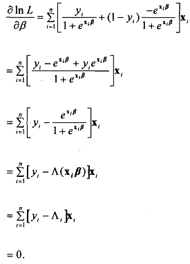
Substituting in (12.25) we have

Notice that the structure of this equation is very similar to the normal equation n obtained for the classical linear model. There we had  and here we have
  . In that context we may interpret the term in square r=l brackets as a residual of sorts.
The second, order conditions for a maximum will always hold in the case of the logit and probit models as the probability density functions of both the normal and the logistic distributions are globally concave.