Baumol's Static Model:

Assumptions

1) Time-horizon of a firm is a single period.

2) The firm maximises total sales revenue subject to a profit constraint.

3) The minimum profit constraint is exogenously determined by the demands and expectations of the shareholders, banks and other financial institutions.  

4) Cost curves are U-shaped and the demand curve is downward sloping. 

Model 1: A single-product model without advertising

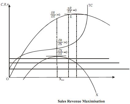
The total cost (TC) and total revenue (TR) curves under the above assumptions are shown below in Figure. The curve (inverted U) below the TR and TC curves is the total profit curve, obtained by deducting TC from  TR for every level of output (X).   

The maximisation of sales revenue for a firm occurs at a point where the marginal revenue equals zero. In the figure, the MR = 0 is attained at a point like E, corresponding to which we have the firm producing OX* level of output. But then whether this maximum sales revenue will be realized or not depends on the level of the minimum acceptable profit, which may act as a constraint to the activity of the firm.  If the minimum acceptable level of profit (π) is 1π , then the firm will produce OX* which will maximise the sales revenue. With OX* output, the firm will actually earn a profit of  . 1 SM π > π In this case, the minimum profit constraint is not operative.  If the minimum acceptable level of profit is , 2π , than the firm will not be able to maximise sales revenue. It would end up at point  E′ on the TR curve where MR > 0, corresponding to which the firm producesOX ′ . In this case, the minimum profit constraint is operative. 

If the profit constraint is operative, the following can be predicted in the single-period model of Baumol:

1)  Sales maximiser produces a higher level of output compared to the profit maximiser. 

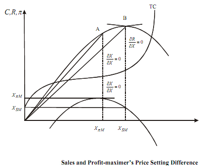
Profit is maximised where ∂π/∂X = 0 corresponding to which we have the output level X_πM. At X_πM , ∂R/∂X = 0, which implies sales revenue is still rising. So that the output level where ∂R/∂X would obviously lie to the right of OX_πM .  Hence X_πM < X_SM

As slope of OA > OB

2) The sales maximiser sells at a price lower than that of the profit maximiser. The price at any level of output is the slope of the ray through the origin to the relevant point of the TR curve. In Figure, the price of profit-maximiser is given by the ray OA and the price of sales maximiser by the ray OB. 

3) The sales-maximiser earns lower  π than that of the profit-maximiser. This is shown in Figure where π_πM > π_SM .

4)  The sales maximiser will never choose a level of output at which price elasticity (e) is less than 1.

Note that

If  |e| < MR < 0 implies TR is declining which is not acceptable for a sales revenue maximising firm. In fact, the firm will choose that level of output where MR = 0 implying |e| = 1, provided the profit-constraint is not operative. If such a constraint is operative the firm would produce where |e|> 1.