Presence of autocorrelation:

Note that the problem of autocorrelation primarily arises in the case of  time series data and not for cross-sectional data. Panel data involves a different set of  tools and are not covered in  this course. It is easiest to make  this point using the consumption function  example. Say consumption  and  income data are  collected across households (cross-sectional data)  for August, 2006. It is extremely unlikely that  the error  terms will be correlated. That  is secause  correlation  usually occurs when there  is  a common event that creates a deviation from the  'truey  model. or 'hstance,  one household holding a party  may be  a reason why their error term may be high (consumption expenditure much higher  than predicted by income and other factors, which are the regressors or  independent variables  in the model estimated). However it is extremely unlikely that just because bouseliold i had a party, household  j will also  have a party during the same time period, when data was collected. Note that if all households are having a party during the survey period then this is a common factor for all data points and gets captured in  the intercept term in the model (given income and other factors, consumption is predicted to be higher for all), and this does not affect the error terms.  

For  time  series data, however, there  is usually  considerable inertia; most macroeconomic time series data follow a cyclical behaviour due to business cycles. For  several periods  income and consumption will be  low; then income  starts recovering. However, consumption shows an inertia and recovers after a lag as people become more confident  that  the rise in incomeis nJot  temporary but permanent and change their consumption patterns slowly over time. In terms of the error term this will show  up as  several consecutive data points with low errors (deviations  from the estimated model), then several periods when  the errors are large (due to the inertia in economic behaviour), and  so on. 

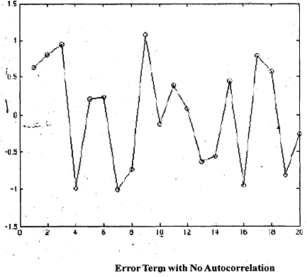
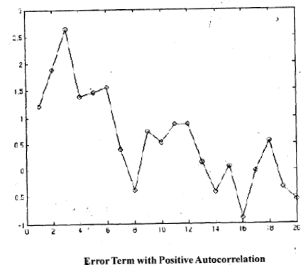
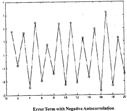
In Fig.1, Fig.2 and Fig.3 we show different error terms, the true values, Note that the  true values  of error  terms are  not observable  and are given here for illustrative purposes. In reality you will observe only the estimated residuals from the MRM. First,  in  Fig.1  there  is no  autocorrelation.  In Fig.2, there is positive autocorrelation  in  the error  structure. Finally, in Fig.3 there  is negative autocorrelation. In the first figure you will find that the error terms are scattered around zero, which is expected, since it is a normal variable drawn independently with mean zero. Hence, there should be no correlation between consecutive error terms. So a plot should not reveal any pattern at all. In Fig.2 on  the other hand there is substantial correlation between the error  terins in consecutive periods; there are several periods when the error is high followed by  several periods when it is low. So there is a  cyclical pattern to be observed  in  the plot of residuals. This  is true for most time series obtained from the real world, i.e., this is the most common pattern.  Fig.3 shows negative autocorrelation. This shows period  to period fluctuations,  that is, if  this period the error is highly positive the next period it will be highly negative and the period after that it will be highly positive again. In other words, consecutive  terms are correlated but the  sign changes from positive to negative and back and so on.

Fig.1

Fig.2

Fig.3