Autocorrelated Error:

To make this discussion more  concrete, we now consider a specific example. In order  to be more specific that we are dealing with time series data we use the subscript 't' instead of 'i'.  

Let us assume that the error term is generated by  the following mechanism

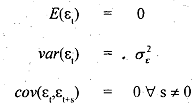
where p is also known as the coefficient of autocovariance and where E,  is the stochastic error term such that it satisfies the standard OLS assumptions, namely,

which says that &term  has constant mean, fixed variance  and is independent,  not correlated with any othervalue  of the  time series E_s.  The technical  term for  the error generation scheme that we have assumed is aJirst  order autoregressive scheme, usually denoted as AR(1) (more details on this are given in Unit on  time series).Given  this'scheme, it can be shown (derivations have been skipped for simplicity),
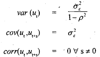
that

where corr(xy)  denotes correlation between variables x and y. Note first that the variance of the error  tern  are fixed.  Second, the error term is correlated  not only with  its immediate past value but also several period's past value as well. It is  important to note that it always needs  to be that |p|<l,  that is, theabsolute value of p  is  less an one. If for example p=l then  the variances and covariances above are not defined.' Under  this assumption also note that the value of the covariance declines as we go further into the past.  .

There are  two reasons for using this process (first order autoregressive). First, it is the simplest  form of a correlated  error  term structllre. Second, it is  the most widely used in terms of applications. A considerable ammount  of theoretical and empirical work has been done using such processes. The reasons for using the ,first order autoregressiGe process are both because it is the simplest form of a correlate&error  term structure,  as well as  it is  the most widely used  in terms of applications. A considerable amount of theoretical and empirical work has been done using such processes.

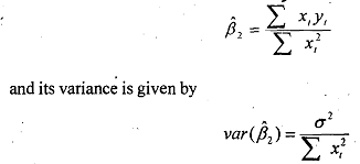
where y_t  is the deviation from the sample mean, that is y_t =  (y_t  - y')  given that y' is the mean value of y_t,  and similarly  for x_i. Now it can be shown under this error scheme that the variance of the OLS estimator is

Note the difference between the variance of the OLS estimator under standard assumptions of no autocorrelation  in the new variance of the estimator with autocorrelation (in the  form of a  first order  autoregressive  error  term)'. The former is added by a factor which is  the multiple of p as well as the sample autocorrelation between the values  taken by the regressor  X  at various lags. Note that if p  is zero then there is no autocorrelation which means that the two values will coincide as expected. We  cannot say whether the former is smaller or bigger than the latter, but that they are different. Note in this context  that for most economic time series data it is not unreasonable  to assume that the regressors are positively  correlated (consumption high in one period usually means  it will be high in the next period as well), rarely do economic data follow a period  to period fluctuations. Usually they  follow a cycle (high values for a while 'during boom, followed by average and then  low values during  recession) wllich leads  to positive correlation between successive values of  the time series.