Vector operations:

As vectors are special cases of matrices, the matrix operations elaborated (addition, subtraction, multiplication, scalar multiplication, transpose) work on vectors and also as the dimensions are right.

For vectors, we know that the transpose of a row vector is the column vector, and the transpose of a column vector is a row vector.

To multiply vectors, they should have similar number of elements, but one should be a row vector and the other a column vector. For illustration, for a column vector c and row vector r:

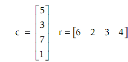
Note that r is a 1 × 4, and c is 4 × 1. Recall that to multiply the two matrices,

[A]_{m ×n} [B]_{n ×p} = [C]_{m × p}

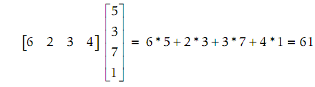
Therefore [r] _1×4 [c] _{4 × 1} = [s] _{1 × 1}, or in another word a scalar:

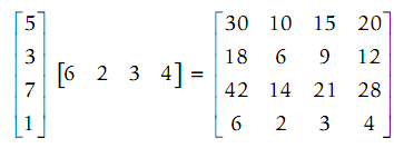
While [c] _{4 × 1} [r] _{1 × 4} = [M] _{4 × 4}, or in another words a 4×4 matrix:

In a MATLAB, such operations are accomplished by using the * operator, that is the matrix multiplication operator. At first, the column vector c and row vector r are generated.

>> c = [5 3 7 1]';

>> r = [6 2 3 4];

>> r*c

ans =

         61

>> c*r

ans =

30 10 15 20

18  6  9 12

42 14 21 28

 6  2  3  4