The purpose of this assignment is to use Matlab/Simulink to analyse and simulate a mathematical model of an electromechanical system. This system comprises two component subsystems consisting of the electrical circuit and translational mechnical system shown in Figure.

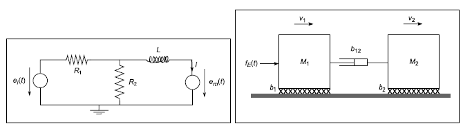
Figure: The two component subsystems of an electromechanical system.

The coupling is through the voltage source em(t) (and current i) and the applied force fE(t) (and the velocity v1) and will be considered later in the assignment. We will first analyse the two subsystems separately.

For the entire assignment let α denote the last digit of your ID number (the large seven digit number across the front of your university card). This parameter will be used to personalise some of the constants used in the assignment. Ensure that you use the last digit of your own ID number!

1. Considering the electrical system in Figure 1(a) in isolation first: There are two inputs to the system consisting of the voltage sources ei(t) and em(t) and the output is the current i(t).

(a) Obtain a system model of this electrical system as a single differential equation (in i,em and e2) coupled with a single alegbraic equation in i, ei and e2, where e2 denotes the voltage across the resistor R2. Construct a continuous-time Simulink modelfor the electrical system when the two inputs are step functions of the form:

(b) Simulate your model using a unit step input at time t = 1 s for ei(t) only (e0 = 1, e1 = 0, τ0 = 1), investigating the transient and steady state parts of the response (for current, i), using the appropriate parameter values from Table 1 (use the values in the column corresponding to your value for α). Then explore the effects of varying R1 and L independently. Explain your results.

(c) Simulate your model using a unit step input at time t = 1 s for em(t) only (e1 = 1, e0 = 0, τ1 = 1), investigating the transient and steady state parts of the response (for current, i), using the the appropriate parameter values from Table 1. Then explore the effects of varying R1 and L independently. Explain your results and compare them with those obtained in Part 1(b).

(d) Simulate your model using a unit step input at time t = 1 s for e0(t) and a step to 0.75 V at time t = 3 s for em(t) (e0 = 1, e1 = 0.75, τ0 = 1, τ1 = 3), investigating the transient and steady state parts of the response (for current, i), using the appropriate parameter values from Table 1. Explain your results. Then explore the effects of varying τ1 - what general principle (for linear systems) do your results illustrate?

(e) In the case where the input voltage em(t) = 0 derive the transfer function G1(s) relating the input voltage Ei(s) to the output current I(s) (i.e., I(s) = G1(s)Ei(s)). Then plot the unit step response using the Matlab command step and verify your result for Part 1(b).