Sketch the direction field for the subsequent differential equation. Draw the set of integral curves for this differential equation. Find out how the solutions behave as t → ∞ and if this behavior based on the value of y(0) explain this dependency.

y' = (y² - y - 2)(1 -y)²

Solution

First, do not be concerned about where such differential equation arrives from. In fact, we just made it up. This may, or may not explain an actual physical situation.

Such differential equation looks somewhat more complex than the falling object illustration from above. Although, with the exception of a little more work, this is not much more complex. The first step is to find out where the derivative is zero.

0 = (y² - y - 2)(1 -y)²

0 = (y-2) (y + 1) (1 -y)²

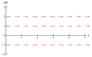
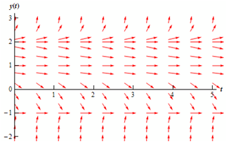
We can here notice that we have three values of y wherein the derivative and thus the slope of tangent lines, will be zero. The derivative will be zero on y = -1, 1, and 2. Thus, let's start our direction field along with drawing horizontal tangents for such values. This is demonstrated in the figure below as:

Here, we require adding arrows to the four regions that the graph is here divided in. For all of these regions I will choose a value of y in that region and plug it in the right hand side of the differential equation to notice if the derivative is negative or positive in that area. Again, to find an exact direction fields you must pick some more over values over the entire range to notice how the arrows are behaving over the entire range.

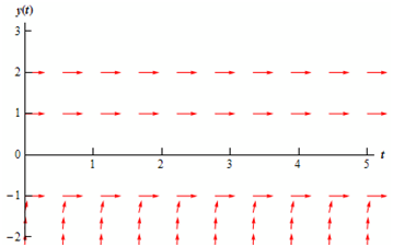
y < -1

In this area we can utilize y = -2 as the test point. At such point we have y′ = 36.  Therefore, tangent lines in that region will have very steep and positive slopes. When also y → -1 the slopes will flatten out whereas staying positive. The figure below demonstrates the direction fields along with arrows in this region.

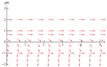
-1 < y < 1

In this section we can utilize y = 0 as the test point. At that point we have y′ = -2.  Thus, tangent lines in that region will have negative slopes and apparently not be extremely steep. Therefore what do the arrows look like in this section? When y → 1 staying less than 1 of course, the slopes must be negative and approach zero. When we move away from 1 and in directions of -1 the slopes will begin to get steeper and stay negative, although eventually flatten back out, again staying negative, when y → -1 as the derivative should approach zero at that point. The figure below demonstrates the direction fields along with arrows added to this region.

1 < y < 2

In this section we will utilize y = 1.5 as the test point. At that point we have y′ = -0.3125.  Tangent lines in this section will also have negative slopes and apparently not be as steep as the earlier. Arrows in this section will behave fundamentally similar as those in the previous. Near y = 1 and y = 2 the slopes will flatten out and when we move from one to the other the slopes will find somewhat steeper before flattening back out. The figure below demonstrates the direction fields along with arrows added to this section.

y > 2

In this last section we will use y = 3 as the test point. At that point we have y′ = 16.  Thus, as we saw in the first region tangent lines will begin out fairly flat near y = 2 and after that as we move way from y = 2 they will find fairly steep.

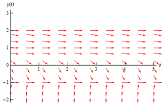
The total direction field for this differential equation is demonstrated below.

There is the set of integral curves for that differential equation. Remember that because of the steepness of the solutions in the lowest section and the software used to make these images I was not capable to comprise more than one solution curve in this area.

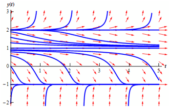
Ultimately, let's take a look at long term behavior of each solution.  Different from the first illustration, the long term behavior in such case will depend on the value of y on t = 0. By examining either of the earlier two figures we can arrive at the subsequent behavior of solutions as t → ∞.

Value of y(0)                           Behavior as t → ∞

y(0) < 1                                    y →-1

1< y(0) < 2                               y → 1

y(0) = 2                                    y → 2

y(0) > 2                                    y→ ∞

Remember to acknowledge what the horizontal solutions are doing. This is frequently the most missed portion of this type of problem.

In both of the illustrations that we've worked to such point the right hand side of the derivative has only comprised the function and NOT the independent variable. As the right hand side of the differential equation comprises both the function and the independent variable the behavior can be much more complex and sketching the direction fields through hand can be very complicated. Computer software is extremely handy in these cases.