Quantity of Pollution Abatement

Let us explain the position through the below diagram using the typical economics analogy. On the x-axis we measure pollution abatement (that is, removal of pollution) by the factory and on y-axis we measure the level of pollution cost. The nearby community faces a downward sloping pollution abatement cost curve (AB).

It indicates that as pollution abatement increases (that is, more amount is pollution is removed or, less amount is pollution is present in the river), there is a decrease in the pollution cost to the community. Thus, when pollution abatement reaches the level 'OB' (that is, all the pollutants are removed from the river), the pollution cost to the community is zero. On the other hand, the factory has an upward sloping pollution abatement cost curve indicating the increasing marginal cost of abatement (OD). When pollution abatement is zero, no pollution cost is borne by the factory.

The factory would like to reduce its pollution abatement expenditure while the community would like the pollution level to be zero. Let us take the situation that the community is holding the property rights for clean environment. Hence, the community can dictate terms to the factory about the pollution load to be released to the river. In this situation, the factory is generating pollution and creating problems for a community that demands zero pollution. For various welfare reasons, the factory cannot be closed down and financial constraints have made the factory to apply limited pollution abatement measures.

In this context, negotiation is the only solution to resolve the conflict. In the negotiation, let us assume that the community can accept a slightly lower Level of pollution emission 'n'. At this level of pollution abatement, however pollution cost to the community is 'h' and pollution cost to the factory is 'g'. Hence, through negotiation, the factory is willing to give compensation up to the extent 'gh' to the community. The level of abatement reached through the negotiation in this case is anywhere between the optimum (t) and the maximum (B).

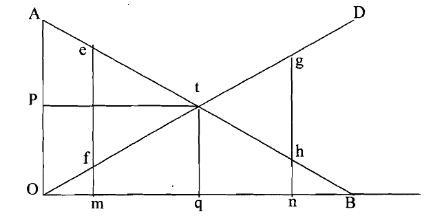
Diagram: Quantity of Pollution Abatement

Let us take the other situation where factory has the property rights. Since the polluter has the property rights, the starting point for negotiation is zero level of pollution abatement. Obviously, for welfare reasons, the community would like the pollution level to be reduced by the factory, which in turn implies higher pollution abatement expenditure by the factory. Suppose the community wants the pollution abatement to be 'm'. At this level, the pollution cost to the community is 'f while pollution abatement cost to the factory is 'e'. It is, therefore, viable to the community to pay compensation to the factory to the extent of 'ef'.

We observe from the above diagram that it is expensive to abate pollution beyond the level 'q'. The government can regulate pollution abatement to be fixed at the level 'q' through command and control measures. Otherwise, it can impose taxes on the polluter (the factory, in this case) to the extent’t’, which is equivalent to the pollution cost on the community. The Coasean principle, however, provides an alternative to pollution tax. Here externality can be internalized through well-defined property rights and compensation.