Learning Weights in Perceptrons

In detail we will look at the learning method for weights in multi-layer networks next chapter. The following description of learning in perceptions will help explain what is going on in the multilayer case. We are in a machine learning set up so we can expect the job to be to learn a objective function which categorizes examples into categories, at least given a set of training examples supplied with their right categorizations. A little thought will be needed in order to select the right way of thinking regarding the examples as input to a set of input units, but, due to the simple nature of a preceptor, there is not much option for the rest of the architecture.

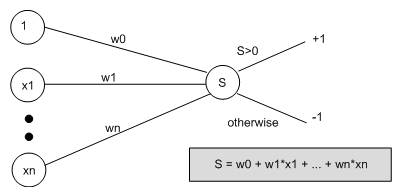
In order to produce a perceptron able to perform our categorization task, we have to use the examples to train the weights among the input units and the output unit, and to train the threshold. To make simple the routine, we think of the threshold as a special weight, that comes from a special input node that always outputs one. Thus, we think of our perceptron like this:

Then, we say that the output from the perceptron is +1 if the weighted sum from all the input units (including the special one) is bigger than zero, and it outputs -1 otherwise. We see that weight w0 is easily the threshold value. Though, thinking of the network like this means in the same way we may train w0 as we train all the other weights.

The weights are first assigned randomly and training instance is used 1 after another to tweak the weights in the network. In the training set all instance are used and the whole process (using all the examples again) is iterated till all examples are exactly categorized by the network. The tweaking is called as the perceptron training rule, and is following like: If the training example, E, is exactly categorized by the network, no tweaking is carried out,then. If E is misclassified, then every specific weight is tweaked by adding on a tiny value, Δ. Imagine we are trying to calculate weight wi, which is between the xi, i-th input unit and the output unit. Then,  given  that  the  network  should  have  calculated  the  target  value  t(E)  for example E, but in fact calculated the observed value o(E), then Δ is calculated as:

Δ = η (t (E) - o (E)) x_i

Notice that η is a fixed positive constant called the learning rate. By ignoring η briefly, we see that the value Δ that we add on to our weight wi is calculated by multiplying the input value xi by t (E) - o (E). t(E) - o(E) will either be -2 or  +2, because perceptrons output only -1 or +1, and t(E) can't be equal to o(E), otherwise we would not be doing any tweaking. Thus, we may think of t(E) - o(E) as a movement in a specific numerical direction, for example, negative or positive. This direction will be like that, if the whole sum, S, was too low to get over the threshold and produce the right categorisation, then the contribution to S from wi * xi will be increased. On the other hand, if S is too high, the contribution from wi * xi is reduced. Because t (E) - o (E) is multiplied by xi, then if xi is a high value (positive or negative), the change to the weight will be larger. To get a better comfort for why this direction correction works, it is a good idea to do some simple calculations by hand.

η simply controls how far the correction should go at 1 time, and is generally set to be a fairly low value, for example, 0.1. The weight learning problem may be seen as finding the global minimum error, calculated as the proportion of miscategorised training examples, over a space where every input values may vary. So, it is possible to move too far in a direction and improve one specific weight to the detriment of the whole sum: while the sum can work for the training example being looked at, it can no longer be a good value for categorizing all the examples correct. Due to this reason, η limit the amount of movement possible. If a large movement is really required for a weight, then it will happen over a series of iterations through the example set. For Sometimes, η is set to decay as the number of such type of iterations through the complete set of training examples increases, so that it may move more slowly towards the global minimum in order not to overshoot in 1 direction. This type of gradient descent is at the heart of the learning algorithm for multi- layered networks, as discussed in the next chapter.

Perceptrons with step functions have restricted abilities when it comes to the range of concepts that may be learned, as discussed in a later section. One way to get better matters is to replace the threshold function with a linear unit, so that the network outputs a real value, rather than a -1or +1. This enables us to utilize another rule, called the delta rule, which is also depending on gradient descent. We do not look at this rule here, because the back propagation  learning  method  for  multi-layer  networks  is same.