Income and Substitution Effects of a Price Change

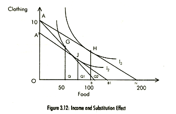
Indifference curve analysis can be used to separate the income effect (IE) from substitution effect (SE). This is shown in Fig. 3.12. When Pc = Rs 60, P_f = Rs 6 and the money income is Rs 600, the consumer is in equilibrium at point G, consuming 50 units of food. When P_f = Rs 3, the consumer is in equilibrium at point H consuming 100 units of food. The increase in demand for food from 50 to 100 units represents combined effect of the substitution and income effect i.e. the price effect (PE). The substitution effect postulates that when the price of food falls, the consumer will substitute food for clothing. On the other hand, the income effect arises because the individuals' real income increases with a fall in P_f and P_c and his income remaining constant so he purchases more food.

To separate the substitution effect form the income effect, we draw hypothetical budget line A¹B¹ tangent to indifference curve 12 at point J. (Note that we have taken Hicksian approach to split the price effect). This budget line involves a reduction in money income, for example by imposing taxes, in order to keep the individual at the same level of real income that he had before the price change. That is, to keep the individual on the indifference curve I₂, The movement along the indifference curve I₂ from G to J (QQ₁ = 25 units of food) is then the substitution effect of the price change, while the shift from point J to H (Q₁Q₂ = 25 units of food) is income effect. The sum of both the effects is the price effect (QQ₂ = 50 units).

It should be noted that the two effects are equal in the example but in the real world the SE is usually larger than the IE. The reason is that the consumer generally spends only a small proportion of his income on anyone good. Thus, even a larger change in the price of the good does not result in a large IE. On the other hand, the SE can be very large if the good has many substitutes.

The SE is always negative, that is, a fall in price of a good will surely result in an increase in demand. But the impact of IE can be positive or negative. This gives rise to three possible situations:

(a)     For normal goods, both the SE and IE reinforce each other. With a fall in price of a good SE is negative and IE is positive. This will definitely increase the demand, therefore, the demand curve will be downward sloping,

(b)     For inferior goods, if the SE is greater than the IE, the demand curve will still be downward sloping, and

(c)     For inferior goods, known as giffen goods, the negative income effect dominates the substitution effect. As a result, the demand curve will be upward sloping.