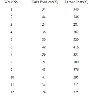
Illustration of Standard error of estimate

The production manager of XYZ Company is concerned about the apparent fluctuation in efficiency and wants to determine how labour costs (in Sh.) are related to volume. The following data presents results of the 12 most recent weeks.

    = 48.95

The sample size, n, is reduced by 2 because 2 variables ‘a’ & ‘b’ in the regression equation had to be estimated from the sample observations.

The calculation of the standard error is necessary because the least square line was calculated from sample data. The other samples would most likely outcome in different estimates. Obtaining the least square calculation over all the possible observations that might occur would result in the calculation of the true least square line. The question is “How near does the sample estimate of least square line come to the accurate least square line.

Standard error is similar to standard deviation in normal probability analysis. This is a measure of variability about the regression line. The std error of estimates enables us to establish a variety of values of the dependent variable in which we may have some degree of confidence that the true value lies. We can use the following equation to establish this range:

Y – tcSe  ≤Y ≤ Y + tcSe

From the above ill, where Y34 = 284.48, the 95% confidence interval can be calculated as follows:

284.48 - 2.2281(48.95)   ≤ Y ≤ 284.48 + 2.2281 (48.95) ≤ Y ≤ 393.6

We are 95% confident that if X is estimated to be 34 units next period, the true labour cost will lie between 175.4 and 393.6.  Note tc from the student T tables, with 10 degrees of freedom and 5% significance level, is equal to 2.2281.