Example of simple exponential smoothing:

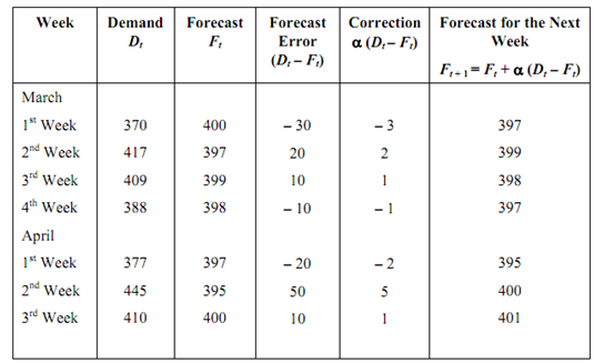
A TV manufacturer utilizes simple exponential smoothing with α = 0.1 to forecast demand. For the first week of March, the forecast was 400 units while actual demand turned out to be 370 units.

1. Forecast the demand for the second week of March.

2. If the actual demand for the second week turned out to be 417 units, forecast the demand for the 3^rd week. Continue forecasting for the subsequent four weeks. You can take actual demands for the subsequent weeks as 409, 388, 377, 445, and 410 units.

3. Develop an adjusted exponential forecast for this company. You may assume the initial trend adjustment factor T_t as zero and β = 0.1.

Solution

(a) F_{t + 1} = F_t + α (D_t - F_t)

                     = 400 + 0.1 (370 - 400) = 397 units.

 (b)

(c)        The trend adjustment is accomplished by total of a correction factor

[(( 1 -β )/ β ) T_{t +1} )]   to the simple exponential forecast.

As the initial trend adjustment factor (given) T_t = 0, we have

March 1^st Week

T_{t + 1} = β (F_{t + 1} - F_t) + (1 - β) T_t

= 0.1 (397 - 400) + (0.9) (0) = - 0.30

T_{(t +1) adj} = F_{t +1} +( 1 -β / β )T _{t +1}

= 397 +( 0.9/0.1)  (- 0.30) = 394.30

The adjusted forecast for the second week of March = 394.30.

March 2^nd Week

T_{t + 1} = 0.1 (399 - 397) + (0.9) (- 0.30)

= 0.2 - 0.27 = - 0.07

F_{(t + 1) adj} = 399 + 9 (- 0.07) = 398.37

The remaining values may be put in table form, as below.

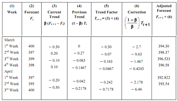
The trend-adjusted forecast for the third week of April is F_{t, adj}   = 393.54 units whereas simple exponential forecast for the same week is 400 units.

The main reason for broad use of simple and adjusted exponential smoothing is that the forecast may be computerized quickly, requires very little memory space, and data can be updated easily. These methods are specifically useful to firms which have thousands of items in inventory. Since each forecast value contains all past forecast and demand data in the properly exponentially weighted manner, there is no requirement to maintain records of historical data (as in case of arithmetic moving averages). It is an effective and efficient method of forecasting with a built-in means of tracking the average while discounting the erratic random fluctuations.