In the earlier section we modeled a population depends on the assumption that the growth rate would be a constant. Though, in reality it doesn't make much sense. Obviously a population cannot be permitted to grow forever at the same rate. The growth rate of population requirements to depends on the population itself. One time a population reaches a certain point the growth rate will start decrease, frequently drastically. A much more realistic model of a population increase is specified by the logistic growth equation.  Now there is the logistic growth equation is,

P' = r (1 -( P/K))P

In the logistic growth equation r is the intrinsic growth rate and is similar r as in the last section. Conversely, it is the growth rate which will arise in the absence of any limiting factors. K is termed as either the saturation level or the carrying capacity.

Here, we claimed that it was a more realistic model for a population. Here we see if that in fact is accurate. To permit us to sketch a direction field let's choose a couple of numbers for r and K.  We'll utilize r = ½ and K = 10. For these values the logistics equation is as:

P' = ½ (1 - (P/10)) P

If you require a refresher on sketching direction fields go back and take seem that section.  Firstly observe that the derivative will be zero at P = 0 and P = 10.  Also see that these are actually solutions to the differential equation. These two values are termed as equilibrium solutions as they are constant solutions to the differential equation. We'll put down the rest of the details on sketching the direction field for you. Now there is the direction field and also a couple of solutions sketched in also.

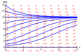
Remember that we comprised a small portion of negative P's in here even if they really don't make any logic for a population problem.  The purpose for this will be apparent down the road. Also, see that a population of as 8 doesn't make all that much logic so let's suppose that population is in thousands or millions hence 8 actually shows 8,000 or 8,000,000 individuals in a population.

See that if we begin with a population of zero, there is the population stays at zero and is no growth. Thus, the logistic equation will properly figure out that.  Subsequently, notice that if we begin with a population in the range 0 < P(0) < 10 so the population will grow, but begin to level off once we cluster to a population of 10. If we begin with a population of 10, the population will continue at 10. At last if we begin with a population which is greater than 10, then the population will in fact die off until we begin nearing a population of 10, at that point the population decline will come to slow down.

Here, from a realistic standpoint this must make some sense. Populations cannot just grow forever without bound. Finally the population will arrive at such a size which the resources of an area are no longer capable to sustain the population and the population growth will start to slow as this comes closer to such threshold.  As well as, if you start off with a population greater than what a region can sustain there will in fact be a die off till we get near to this threshold.

In this case that threshold shows to be 10 that is also the value of K for our problem. That must explain the name which we gave K initially. The saturation level or carrying capacity of an area is the maximum sustainable population for such area.

Therefore, the logistics equation, whereas still fairly simplistic, does an excellent job of modeling what will occur to a population.

Here, let's move on to the point of such section. The logistics equation is an instance of an autonomous differential equation. Autonomous differential equations are differential equations which are of the form.

dy/dt = f(y)

The only place that the independent variable, t in this case, appears is in the derivative.

Note thee that if f (y₀) = 0 for some value y = y₀ so this will also be a solution to the differential equation. These values are termed as equilibrium solutions or equilibrium points. What we would like to do is categorize these solutions. Through classify we mean the subsequent. If solutions begin "near" an equilibrium solution will they move away from the equilibrium solution or in the directions of the equilibrium solution? Upon classifying the equilibrium solutions we can after that knows what all the other solutions to the differential equation will act in the long term simply through looking at those equilibrium solutions they start near.

Thus, just what do I mean by "near"?  Go back to our logistics equation.

P' = ½ (1 - (P/10))P

When we pointed out there are two equilibrium solutions to such equation P = 0 and P = 10.  If we avoid the fact that we're dealing along with population these points break-up the P number line in three distinct areas.

-∞ < P < 0,                  0< P < 10,                    10 < P < ∞

We will say that a solution begins "near" an equilibrium solution whether it begins in a region which is on either side of that equilibrium solution. Thus solutions which start "near" the equilibrium solution P =10 will start in either

0 < P < 10        OR       10 < P < ∞

And solutions which start "near" P = 0 will start in either

-∞ < P < 0, or 0 < P < 10

For regions which lie between two equilibrium solutions we can imagine any solutions starting in such region as starting "near" either of the two equilibrium solutions as we require to.

Here, solutions that start "near" P = 0 all move ahead of the solution as t rises. Note that moving away does not essentially mean that they grow without bound as they diverge.  It only means that they move away. Solutions which start out greater than P = 0 move away, but do stay bounded like t grows. Actually, they move in towards P = 10.

Equilibrium solutions wherein solutions that start "near" them move away by the equilibrium solution are termed as unstable equilibrium points or unstable equilibrium solutions.  Thus, for our logistics equation, P = 0 is an unstable equilibrium solution.

Subsequently, solutions that start "near" P = 10 all move in the direction of P = 10 as t raises. Equilibrium solutions wherein solutions that start "near" them move in the direction of the equilibrium solution are termed as asymptotically stable equilibrium points or asymptotically stable equilibrium solutions. Therefore, P = 10 is an asymptotically stable equilibrium solution.

Here is one more classification, but I'll wait till we get an example wherein this occurs to introduce this. Hence, let's take a look at a couple of illustrations.