Derivation Of Ordinary Demand Function:

Suppose,  and q₁ = (Q₁¹, Q₂¹,..., Q_n¹)T. Let M0 be the money income and p₀q₀ = M₀ and p₀q₀≥ p₀q₁, where p₀q₁ is the total expenditure of buying q1 at p0 set of prices. q0 is revealed preferred to q1. Let the set of prices when she buys q₁ be p₁ = (p₁¹, p₁²,..., p₁ⁿ), then q₀ is not an available alternative at p1 price. p₁q₁1q₀ and M₁1q₀. 

For simplicity lets consider a two-goods world and at initial prices and money income, budget line is AB, which is shown in the following figure.  According to the axiom, budget line is downward sloping and linear. Suppose the consumer chooses the bundle (x₁⁰, x₂⁰). Moreover suppose that for given money income M and price of the good two (viz. p₂) (i.e., given the intercept of the budget line) p₁ decreases. Then  would fall. Now initial budget line is AB becomes flatter with same intercept. None of the commodity bundles on the new budget line are previously available. Therefore, according to weak axiom of revealed preference, consumer can choose any commodity bundle from the new budget line AC. Suppose it is at point V. That means ordinary demand curve can take any algebrical slope. In this case, x₁ increases due to fall in p1 for given p₂ and M. Ordinary demand curve is downward sloping or, own price effect is negative. Let us show that this own price effect consists of own substitution effect and income effect for a price change by using Slutsky's method, where real income is measured in terms of purchasing power. Given the money income, as p₁ decreases, real income increases by which demand for x₁ changes. To ignore this, money income reduces proportionately so that real income in terms of purchasing power is constant i.e., after adjustment of money income, the budget line AC shifts parallely downward such that it passes through the original commodity bundle i.e., point z to maintain same purchasing power.   

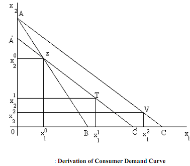
 Such a budget line is known as compensated budget line along which real income (in terms of purchasing power) is constant. This is denoted by line A'C' in the diagram. Note that the consumer always chooses a commodity bundle only from the compensated budget line A'C'. But according to weak axiom of revealed preference, consumer can't choose any bundle between A'z since all these bundle are previously available at the budget line AB. But consumer doesn't prefer these as she preferred the bundle z. Therefore, consumer can choose any bundle in between z and C' under constant real income. If the consumer chooses the bundle z, then we have a single quantity of good 1 with two different prices which is not possible in view of the fact that the demand function is single valued. Hence, under the constant real income consumer actually chooses any bundle on the line A'C' right to the point z, say at point T.