Let us consider a bond with callable or prepayable feature. Figure shows the price/yield relationship of option-free bond and callable bond. The price yield relationship of option-free bond is represented by the convex curve a - a'. The price yield relationship of the callable bond is represented by the unusual curve a -b.

When market yield for comparable bonds is higher than the coupon rate on the callable bond then issuer will not call the bond. For example, if the coupon rate on a bond is 8% and the prevailing market yield on comparable bond is 13%, then undoubtedly issuer will not call the bond. Because the issuer of the bond is unlikely to call it, the price/yield relationship of callable bond is equal to the option-free bond. Therefore, the callable bond is valued as an option free bond. However call option still has some value, so the bond is not exactly priced like an option free bond.

If yield decreases in the market then there is a chance that issuer will call the bond. It is not necessary that issuer exercise the call option as market yield drops below the coupon rate. However, as yield approaches the coupon rate from higher yield level, the value of the embedded option increases. For example, assume that yield decreases from 13% to 8.75%; then it is most likely that issuer will not exercise the call option. But the issuer would probably exercise his right to call if the market yield declines further. The call option becomes more valuable to the issuer in this circumstance, thus reducing the price of the callable bond when compared to that of a comparable option-free bond. In figure 5, the value of the embedded call option at a given yield can be measured by the difference between the price of an option-free bond and the price on the curve a - b. We can also notice that at low yield levels, the value of the embedded call option is high.

Let us see how the price volatility property of a callable bond is different from that of an option-free bond. Figure 6 magnifies the portion of the price/yield relationship for the callable bond where the two curves in the figure depart. (Segment b - b' in figure ). As per property 4, when there is a large change in yield of a given number of basis points, the price of an option-free bond increases more than it decreases. But in case of a callable bond, the opposite is true i.e. for a given large change in the yield, the price of the bond appreciation is less than the price decline.

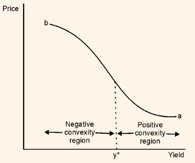
Let us look into the price volatility characteristic of a callable bond. From figure 1 it is clear that the curve has a concave shape. In financial terms, this is referred to as negative convexity. This characteristic of callable bond is not exhibited at every yield level.

When yield is high (in comparison to coupon rate), the bond shows same price/yield relationship as an option-free bond; and therefore at this level the gain is greater than the loss. The price/yield relationship of a option-free bond is referred to as positive convexity. Therefore, for a callable bond, we see negative convexity character at low yield levels and positive convexity character at high yield levels. This is illustrated in figure 2.

Figure 1: Negative Convexity Region of the Price/Yield Relationship for a Callable bond

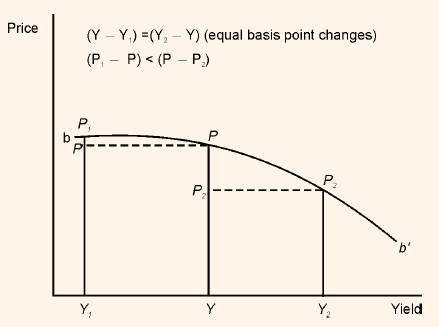
Figure 2: Negative and Positive Convexity Exhibited by Callable bond

We see in Figure 7 that at certain yield levels, when rates decline there is very little price appreciation. A bond is said to exhibit "price compression," when it enters this region.