The option features embedded in many bonds and fixed-income securities have made the binomial interest rate tree approach a valuable model for pricing debt. Binomial model is an option valuation method developed by Cox, Ross, Rubinstein and Sharpe in 1979. This method of pricing options or other equity derivatives is based on the assumption that probability of each possible price follows a binomial distribution and that prices can either move to a higher level or a lower level with time until the option expires.

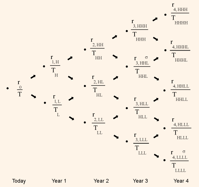
To value bonds using the binomial model, a binomial interest rate tree is to be constructed first. A binomial interest rate tree is nothing but a graphical representation of the short-term interest rates over a period of time based on some assumption about interest rate volatility. In this tree, each node represents a defined time period, say one year. Each node is represented by the letter T. The current year spot rate for the specified time period, in our example one-year spot rate, is represented by r₀. As the model is based on the assumption that each possible price can either move higher or lower, each node gives rise to two options, T_H and T_L, where H represents higher and L represents lower. (Multiple paths to same node have been avoided to keep the figure simple. For example, HL can be reached in two ways, HL and LH, but only HL is shown in the Table.)

In Table 1, we see that T is the starting point of the interest rate tree, and r₀ represents the current 1-year spot rate. It is assumed that the 1-year rate can take two possible values, either higher or lower, in the defined time period, i.e., 1-year in our example and they both have the same probability of occurrence.

         σ       = Assumed volatility of the 1-year rate.

         r_{1, L}      = The lower 1-year rate one year from now.

         r_{1, H}      = The higher 1-year rate one year from now.

Table 1: Binomial Interest Rate Tree

Now, we can define the relationship between the lower and higher value as follows:

r_{1, H} = r_{1, L} ( e ^2σ)

e is the base of the natural logarithm, 2.71828.

Let us calculate the values using a hypothetical example; let us assume that the value of r_{1, L} to be 4.7801, σ is 10% per year, then,

r_{1, H} = 4.7801% (e ^2*0.10) = 5.8384

In the second year, we find three possible values for the one year rate; they are:

r_{2, HH}  =      1-year rate in second year assuming the higher rate in the first year and the

 higher rate in the second year.

r_{2, HL}   =       1-year rate in second year assuming the higher rate in the first year and the

 lower rate in the second year.

r_{2, LL}    =       1-year rate in second year assuming lower rate in first year and lower rate in

 second year.

r_{2, HH}  is defined as r_{2, LL} (e ^{4 σ}) and r_{2, HL} = r_{2, LL}( e ^2σ).

Assuming r_{2, LL} to be 4.8051% and σ as 10%, we can determine r_{2, HH}, r_{2, HL} as follows:

r_{2, HH} = 4.8051% (e ^4*0.10) = 7.1683%

r_{2, HL} = 4.8051% (e ^2*0.10) = 5.8689%

There are four possible values for the 1-year rate in the third year, they are denoted as r_{3, HHH}, r_{3, HHL} , r_{3, HLL} and r_{3, LLL.}

The relationship between them can be expressed as follows:

r_{3, HHH} = r_{3, LLL}( e ^6σ)

r_{3, HHL} = r_{3, LLL}(e ^4σ)

r_{3, HLL} = r_{3, LLL}( e ^2σ).

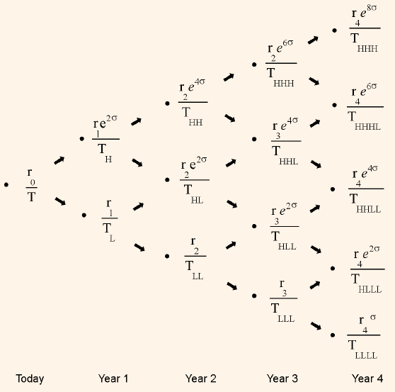
Let us make the Table easier to understand by replacing the notations with the simplified notations.

Table 2: Binomial Interest Rate Tree with One-Year Rates

*rt equals forward 1-year lower rate. t year from now.

In valuing option free bonds, we have seen the use of single forward rate, but in valuing bonds with embedded option we use a set of forward rates, as at every level we come with more then one option.