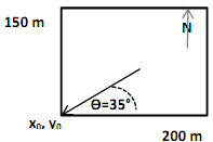
An environmental consulting firm is conducting a site investigation on an abandoned industrial site that is 200 m by 150 m in size (Fig. 1). A number of piezometers were installed on site to obtain information about the subsurface aquifer. Geologic samples were obtained from the drill cuttings and sent for analysis. The hydraulic conductivity of the aquifer solids was found to be 0.32 m/d and the porosity was found to be 0.36.
The groundwater hydraulic gradient was found to be 0.0012, sloped downward to the southwest corner of the site, and oriented at 35 degrees to the southwestern corner of the site. The groundwater head was measured to be 92 m above mean sea level in a piezometer that was located at the southwest corner of the site. The general relationship between head and location in a 2-dimensional aquifer is as follows:

Where H(x0,y0) is the head measured at the location (x0,y0), θ is the angle that the hydraulic gradient makes with the line y=y0 (i.e., the horizontal line that intersects x0, y0), dh/dl is the magnitude of the hydraulic gradient. The following plan view represents information about the hydraulic gradient at the site:
.a. Sketch a flowsheet of the steps that you would take to simulate the groundwater aquifer at this site by calculating the groundwater head with a spatial resolution of 1 meter in the x-direction and 1-meter in the y-direction. Be sure to note how you plan to organize data with scalar, vector and matrix elements.
b. Write a well-documented MATLAB program to simulate the groundwater aquifer at this site by calculating the groundwater head with a spatial resolution of 1 meter in the x-direction and 1 meter in the y-direction. You should explain the rationale for any supporting calculations or assumptions made.
c. Create a contour plot of head values in the x-y plane (See MATLAB Quick Tips for syntax in creating plot). This plot is a 'bird's-eye' view of the topographical contours of constant head on the water table.
d. Create a transect (also called cross-section) plot showing the vertical head as a function of distance:
i. In the x-direction, at a distance of 30 m north of the southwest corner of the site.
ii. In the y-direction, at a distance of 56 m east of the southwest corner of the site.