Approximating solutions to equations newtons method, Mathematics

Assignment Help:

Approximating solutions to equations : In this section we will look at a method for approximating solutions to equations. We all know that equations have to be solved on occasion and actually we've solved out quite a few equations by ourselves to this point.  In all the instances we've looked at to this instance we were capable to in fact find the solutions, however it's not always probable to do that exactly and/or do the work by hand.

That is where this application comes into play.  Therefore, let's see what this application is all about.

1141_Newton’s Method.png

Let's assume that we desire to approximate the solution to f (x) = 0 and let's also assume that we have somehow found an initial approximation to this solution say, x0. This initial approximation is perhaps not all that good and therefore we'd like to discover a better approximation. It is easy enough to do.  Firstly we will get the tangent line to f ( x )at x0.

y = f ( x0 ) + f ′ ( x0 ) ( x - x0 )

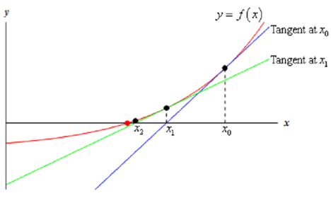
Now, take a look at the graph below.

The blue line (if you're reading this in color anyway...) is the tangent line at x0. We can illustrate that this line will cross the x-axis much closer to the actual solution to the equation than x0 does.  Let's call this point where the tangent at x0 crosses the x-axis x1 and we'll utilizes this point as our new approximation to the solution.

Therefore, how do we determine this point? Well we know it's coordinates, ( x1 ,0) , and we know that it's on the tangent line therefore plug this point into the tangent line & solve out for x1 as follows,

0 = f ( x0 ) + f ′ ( x0 ) ( x1 - x0 )

x - x0 = -  f (x0 ) /f ′ ( x0 )

x1 = x0  - (f ( x0 ) /f ′ ( x0 ))

Therefore, we can determine the new approximation provided the derivative isn't zero at the original approximation.

Now we repeat the whole procedure to determine an even better approximation. We build up the tangent line to f ( x ) at x1 and utilizes its root, that we'll call x2, as a new approximation to the actual solution.  If we do it we will arrive at the given formula.

                  x2= x1 - (f ( x1 ) /f ′ ( x1 ))

This point is also illustrated on the graph above and we can illustrated from this graph that if we continue following this procedure will get a sequence of numbers which are getting very close the real solution. This procedure is called Newton's Method.


Related Discussions:- Approximating solutions to equations newtons method

Describe differance between mean vs. mode, Describe differance between Mean...

Describe differance between Mean vs. Mode ? Every set of numbers or data has a mean and a mode value. The mean is the average value of all the numbers in the set. The mode is t

Differentiate quotient rule functions, Example of quotient rule : Let's no...

Example of quotient rule : Let's now see example on quotient rule.  In this, unlike the product rule examples, some of these functions will require the quotient rule to get the de

Trigonometric ratios, to difine trigonometric ratios of an angle,is it nece...

to difine trigonometric ratios of an angle,is it necessary that the initial ray of the angle must be positive x-axis?

Graph f(x) = ex and g(x) = e- x - common graph, Graph f ( x ) = e x and g ...

Graph f ( x ) = e x and g ( x ) = e - x . Solution There actually isn't a lot to this problem other than ensuring that both of these exponentials are graphed somewhere.

Numerical method, The Stefan-Boltzmann law can be employed to estimate the ...

The Stefan-Boltzmann law can be employed to estimate the rate of radiation of energy H from a surface of copper sphere with radius = 0.15 ±0.01 m, as in H=AesT^4 where H is in watt

Find the total volume of the hay stack, The lower portion of a hay stack is...

The lower portion of a hay stack is an inverted cone frustum and the upper part is a cone find the total volume of the hay stack.

Highest common factor (hcf), We know that a factor is a quantity whic...

We know that a factor is a quantity which divides the given quantity without leaving any remainder. Similar to LCM above we can find a highest common factor (HCF)

Logarithm, The function A(t) = 5(0.7)^t was used to define the amount A in ...

The function A(t) = 5(0.7)^t was used to define the amount A in milliliters of a drug in the bloodstream t hours after the drug was ingested. Determine algebraically the time it wi

Parallel vectors - applications of scalar multiplication, Parallel Vectors ...

Parallel Vectors - Applications of Scalar Multiplication This is an idea that we will see fairly a bit over the next couple of sections.  Two vectors are parallel if they have

Write Your Message!

Captcha
Free Assignment Quote

Assured A++ Grade

Get guaranteed satisfaction & time on delivery in every assignment order you paid with us! We ensure premium quality solution document along with free turntin report!

All rights reserved! Copyrights ©2019-2020 ExpertsMind IT Educational Pvt Ltd