Reference no: EM131097062

10701 Machine Learning - Spring 2012 - Final Examinations

Q1. Decision trees and KNNs

In the following questions we use Euclidian distance for the KNN.

1.1 Assume we have a decision tree to classify binary vectors of length 100 (that is, each input is of size 100). Can we specify a 1-NN that would result in exactly the same classification as our decision tree? If so, explain why. If not, either explain why or provide a counter example.

1.2

Assume we have the decision tree in Figure 1 which classifies two dimensional vectors {X₁, X₂} ∈ R\{A, B}. In other words, the values A and B are never used in the inputs. Can this decision tree be implemented as a 1-NN? If so, explicitly say what are the values you use for the 1-NN (you should use the minimal number possible). If not, either explain why or provide a counter example.

Q2. Neural Networks

Consider neural networks where each neuron has a linear activation function, i.e., each neurons output is given by g(x) = c+b 1/n _i=1∑ⁿW_ix_i, where b and c are two fixed real numbers and n is the number of incoming links to that neuron.

1. Suppose you have a single neuron with a linear activation function g() as above and input x = x₀, . . . , x_n and weights W = W₀, . . . , W_n. Write down the squared error function for this input if the true output is a scalar y, then write down the weight update rule for the neuron based on gradient descent on this error function.

2. Now consider a network of linear neurons with one hidden layer of m units, n input units, and one output unit. For a given set of weights w_k,j in the input-hidden layer and W_j in the hidden-output layer, write down the equation for the output unit as a function of w_k,j , W_j, and input x. Show that there is a single-layer linear network with no hidden units that computes the same function.

3. Now assume that the true output is a vector y of length o. Consider a network of linear neurons with one hidden layer of m units, n input units, and o output units. If o > m, can a single-layer linear network with no hidden units be trained to compute the same function? Briefly explain why or why not.

4. The model in 3) combines dimensionality reduction with regression. One could also reduce the dimensionality of the inputs (e.g. with PCA) and then use a linear network to predict the outputs. Briefly explain why this might not be as effective as 3) on some data sets.

Q3. Gaussian mixtures models

3.1 The E-step in estimating a GMM infers the probabilistic membership of each data point in each component Z: P(Z_j|X_i), i = 1, ..., n, j = 1, ..., k, where i indexes data and j indexes components. Suppose a GMM has two components with known variance and an equal prior distribution

N(µ₁, 1) × 0.5 + N(µ₂, 1) × 0.5                                                                      

The observed data are x₁ = 2, and the current estimates of µ₁ and µ₂ are 2 and 1 respectively. Compute the component memberships of this observed data point for the next E-step (hint: normal densities for standardized variable y_(µ=0,σ=1) at 0, 0.5, 1, 1.5, 2 are 0.4, 0.35, 0.24, 0.13, 0.05).

3.2 The Gaussian mixture model (GMM) and the k-means algorithm are closely related-the latter is a special case of GMM. The likelihood of a GMM with Z denoting the latent components can be expressed typically as

P(X) = ∑_zP(X|Z)P(Z)

where P(X|Z) is the (multivariate) Gaussian likelihood conditioned on the mixture component and P(Z) is the prior on the components. Such a likelihood formulation can also be used to describe a k-means clustering model. Which of the following statements are true-choose all correct options if there are multiple ones?

a) P(Z) is uniform in k-means but this is not necessarily true in GMM.

b) The values in the covariance matrix in P(X|Z) tend towards zero in k-means but this is not so in GMM.

c) The values in the covariance matrix in P(X|Z) tend towards infinity in k-means but this is not so in GMM.

d) The covariance matrix in P(X|Z) in k-means is diagonal but this is not necessarily the case in GMM.

Q4. Semi-Supervised learning

4.1 Assume we are trying to classify stocks to predict whether the stock will increase (class 1) or decrease (class 0) based on the stock closing value in the last 5 days (so our input is a vector with 5 values). We would like to use logistic regression for this task. We have both labeled and unlabeled data for the learning task. For each of the 4 semi-supervised learning methods we discussed in class, say whether it can be used for this classification problem or not. If it can, briefly explain if and how you should change the logistic regression target function to perform the algorithm. If it cannot, explain why.

1. Re-weighting

2. Co-Training

3. EM based

4. Minimizing overfitting

4.2 Assume we are using co-training to classify the rectangles and circles in Figure 2 a). The ? represents unlabeled data. For our co-training we use linear classifiers where the first classifier uses only the x coordinate values and the second only the y axis values. Choose from the answers below the number of iterations that will be performed until our co-training converges for this problem and briefly explain:

1. 1

2. 2

3. more than 2

4. Impossible to tell.

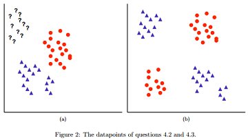
4.3 Now assume that we are using boosting (with linear classifiers, so each classifier is a line in the two dimensional plane) to classify the points in Figure 2 b). We terminate the boosting algorithm once we reach a t such that ∈_t = 0 or after 100 iterations. How many iterations do we need to perform until the algorithm converges? Briefly explain.

1. 1

2. 2

3. more than 2

4. Impossible to tell.

Q5. Bayesian networks

5.1 1. Show that a b, c | d (a is conditionally independent of {b, c} given d) implies a b | d (a is conditionally independent of b given d).

2. Define the skeleton of a BN G over variables X as the undirected graph over X that contains an edge {X, Y} for every edge (X, Y ) in G. Show that if two BNs G and G' over the same set of variables X having the same skeleton and the same set of v-structures, encode the same set of independence assumptions. V-structure is a structure of 3 nodes X, Y, Z such as X → Y ← Z.

Hints: It suffices to show that for any independence assumption A B | C (A, B, C are mutually exclusive sets of variables), it is encoded by G if and only if it is also encoded G'. Show by d-separation.

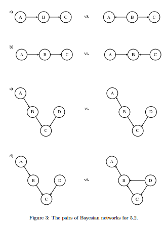
5.2 For each of the following pairs of BNs in Figure 3, determine if the two BNs are equivalent, e.g they have the same set of independence assumptions. When they are equivalent, state one independence/conditional independence assumption shared by them. When they are not equivalent, state one independence/conditional independence assumption satisfied by one but not the other.

5.3 We refer to the Figure 4 in this question.

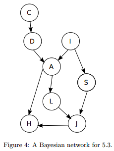
1. What is Markov blanket of {A, S}?

2. (T/F) For each of the following independence assumptions, please state whether it is true or false:

(a) D S.

(b) D S|H.

(c) C J|H.

(d) C J|A.

Q6. Hidden Markov Models

6.1 Assume we have temporal data from two classes (for example, 10 days closing prices for stocks that increased/decreased on the following day). How can we use HMMs to classify this data?

6.2 Derive the probablity of:

P(o₁, . . . , o_t, q_t-1 = s_v, q_t = s_j)

You may use any of the model parameters (starting, emission and transition probabilities) and the following constructs (defined and derived in class) as part of your derivation:

p_t(i) = p(q_t = s_i)

 α_t(i) = p(o₁, . . . , o_t, q_t = s_i)

 δ_i(i) = max_q1,...,qt-1p(q₁, . . . , q_t-1, q_t = s_i, O₁, . . . , O_t)

 Note that you may not need to use all of these constructs to fully define the function listed above.

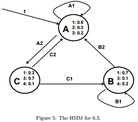
6.3 The following questions refer to figure 5. In that figure we present a HMM and specify both the transition and emission probabilities. Let p^t_A be the probability of being in state A at time t. Similarly define p^t_B and p^t_C.

1. What is p³_C?

2. Define p^t₂ as the probability of observing 2 at time point t. Express p^t₂ as a function of p^t_B and p^t_C (you can also use any of the model parameters defined in the figure if you need).

Q7. Dimension Reduction

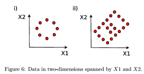
7.1 Which of the following unit vectors expressed in coordinates (X₁, X₂) correspond to theoretically correct directions of the 1st (p) and 2nd (q) principal components (via linear PCA) respectively for the data shown in Figure 6? Choose all correct options if there are multiple ones.

a) i) p(1, 0) q(0, 1) ii) p(1/√(2), 1/√(2)) q(1/√(2), -1/√(2))

b) i) p(1, 0) q(0, 1) ii) p(1/√(2), -1/√(2)) q(1/√(2), 1/√(2))

c) i) p(0, 1) q(1, 0) ii) p(1/√(2), 1/√(2)) q(-1/√(2), 1/√(2))

d) i) p(0, 1) q(1, 0) ii) p(1/√(2), 1/√(2)) q(-1/√(2), -1/√(2))

e) All of the above are correct

7.2 In linear PCA, the covariance matrix of the data C = XT X is decomposed into weighted sums of its eigenvalues (λ) and eigenvectors p:

C = ∑_iλ_ip_ip^T_i

Prove mathematically that the first eigenvalue λ₁ is identical to the variance obtained by projecting data into the first principal component p1 (hint: PCA maximizes variance by projecting data onto its principal components).

7.3 The key assumption of a naive Bayes (NB) classifier is that features are independent, which is not always desirable. Suppose that linear principal components analysis (PCA) is first used to transform the features, and NB is then used to classify data in this low-dimensional space. Is the following statement true? Justify your answers.

The independent assumption of NB would now be valid with PCA transformed features because all principal components are orthogonal and hence uncorrelated.

Q8. Markov Decision Processes

Consider the following Markov Decision Process (MDP), describing a simple robot grid world. The values of the immediate rewards R are written next to the transitions. Transitions with no value have an immediate reward of 0. Note that the result of the action "go south" from state S₅ results in one of two outcomes. With probability p the robot succeeds in transitioning to state S₆ and receives immediate reward 100. However, with probability (1-p) it gets stuck in sand, and remains in state S₅ with zero immediate reward. Assume the discount factor γ = 0.8. Assume the probability p = 0.9.

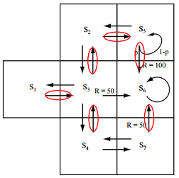
1. Mark the state-action transition arrows that correspond to one optimal policy. If there is a tie, always choose the state with the smallest index.

2. Is it possible to change the value for γ so that the optimal policy is changed? If yes, give a new value for γ and describe the change in policy that it causes. Otherwise briefly explain why this is impossible.

3. Is it possible to change the immediate reward function so that V^∗ changes but the optimal policy π^∗ remains unchanged? If yes, give such a change and describe the resulting changes to V^∗. Otherwise briefly explain why this is impossible.

4. How sticky does the sand have to get before the robot will prefer to completely avoid it? Answer this question by giving a probability for p below which the optimal policy chooses actions that completely avoid the sand, even choosing the action "go west" over "go south" when the robot is in state S₅.

Q9. Boosting

9.1 AdaBoost can be understood as an optimizer that minimizes an exponential loss function E = _i=1∑^Nexp(-y_if(x_i)) where y = +1 or -1 is the class label, x is the data and f(x) is the weighted sum of weak learners. Show that the loss function E is strictly greater than and hence an upper bound on a 0 - 1 loss function E_0-1 = _i=1∑^N 1 · (y_if(x_i) < 0) (hint: E_0-1 is a step function that assigns value 1 if the classifier predicts correctly and 0 otherwise).

9.2 The AdaBoost algorithm has two caveats. Answer the following questions regarding these.

a) Show mathematically why a weak learner with < 50% predictive accuracy presents a problem to AdaBoost.

b) AdaBoost is susceptible to outliers. Suggest a simple heuristic that relieves this.

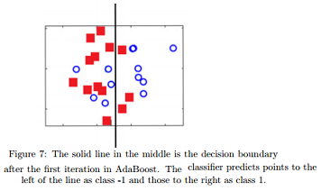
9.3 Figure 7 illustrates the decision boundary (the middle intersecting line) after the first iteration in an AdaBoost classifier with decision stumps as the weak learner. The square points are from class -1 and the circles are from class 1. Draw (roughly) in a solid line the decision boundary at the second iteration. Draw in dashed line the ensemble decision boundary based on decisions at iteration 1 and 2. State your reasoning.