Reference no: EM131231723

Project: Application of Drift-Diffusion Model

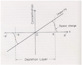
1. This example is a demonstration of the fact that explicit numerical integration methods are incapable of solving even the problem of linearly-graded junctions in thermal equilibrium, for which N_D - N_A = mx   (see Fig. 1) and a is the edge of the depletion region. To demonstrate this, calculate the following:

(a) Establish the boundary conditions for the electrostatic potential [ψ(-a) and ψ(a)] by taking into account the free carrier terms in the equilibrium 1D Poisson equation:

∂²ψ/∂x² = -(e/ε)(p - n + mx) = -(e/ε)(n_ie^-ψ/V_t - n_ie^ψ/V + mx)

(b) Solve analytically the 1D Poisson equation for ψ(x) within the depletion approximation (no free carriers) and calculate a using this result as well as the boundary conditions found in (a). What is the expression for absolute value of the maximum electric field?

(c) Apply the explicit integration method for the numerical solution of the 1D Poisson equations (that includes the free carriers) by following the steps outlined below:

• Write a Taylor series expansion for ψ(x) around x=0, keeping the terms up to the fifth order.
• Starting from the equilibrium Poisson equation, analytically calculate ψ"(0), ψ⁽³⁾(0), ψ⁽⁴⁾(0) and ψ⁽⁵⁾(0).
• Use the maximum value of the electric field derived in (b) to determine, from the Taylor series expansion for ψ(x), the terms ψ(h), ψ(2h) and ψ(3h).
• Compute ψ(x) at x=4h, 5h, 6h, ... , up to xmax = 0.5μm, using the predictor-corrector method in which the predictor formula:

Ψ_i+1 = 2 Ψ_i-1 - Ψ_i-3 + 4h2 (Ψ"_i-1 + (Ψ"_i - 2Ψ"_i-1 + Ψ"_i-2/3))

is applied to predict Ψ_i+1, which is then corrected by the corrector formula:

 Ψ_i+1 = 2Ψ_i - Ψ_i-1 + h²(Ψ"_i + (Ψ"_i+1 - 2Ψ"_i + Ψ"_i-1/12)).

In both, the predictor and the corrector formulas, the second derivatives are obtained from the Poisson's equation. The role of the predictor is to provide   that appears in the corrector formula.

Repeat the above procedure for the following values of the first derivative:

Trial 1: Ψ'(0)₁ = Ψ'(0),

Trial 2:   Ψ'(0)₂ = Ψ'(0)₁/2,

Trial 3: Ψ'(0)₃ = 0.5[Ψ'(0)₁ + Ψ'(0)₂],

 

Trial n: Ψ'(0)_n = 0.5[Ψ'(0)_n-2 + Ψ'(0)_n-1],

where n = 22. Comment on the behavior of this explicit integration scheme. Use the following parameters in the numerical integration:

e = 1.602x10^-19, ε = 12ε₀ = 1.064x10^-12 F/cm, T = 300K,

n_i = 1.4x10¹⁰ cm^-3, m = 10²¹ cm^-4, h = 2x10^-7 cm.  

Figure 1: Linearly-graded junction

Q2. Develop a one-dimensional (1D) drift-diffusion simulator for modeling pn-junctions (diodes) under forward bias conditions. Include both types of carriers in your model (electrons and holes). Use the natural set of variables (potential, electron concentration and hole concentration).

Model: Assume silicon diode, with permittivity ε_sc = 1.05x10^-10 F/m and intrinsic carrier concentration n_i = 1.5x10¹⁰ cm^-3 at T = 300K. In all the simulations assume that T = 300K. Use concentration-dependent and field-dependent mobility models and SRH generation-recombination. Assume ohmic contacts and charge neutrality at both ends, to get the appropriate boundary conditions for the potential and the electron and hole concentrations.

For the concentration-dependent electron and hole mobilities use the Arora model given in the Silvaco Manuals. It will be easier, while you are developing the 1D simulator, to assume constant mobility value for both electrons and holes.

Doping: Use N_A = 10¹⁶ cm^-3 and N_D = 1017 cm^-3, as a net doping of the p- and n-regions, respectively.

Numerical methods: Use the LU decomposition method for the solution of the 1D Poisson and the two 1D continuity equations for electrons and holes individually. Use Gummel's decoupled scheme, described in the class and in the distributed notes, to solve the resultant set of coupled set of algebraic equations.

Outputs:

Plot the conduction band edge under equilibrium conditions (no current flow). You only need to solve non-linear Poisson equation in this case.

Vary the Anode bias V_A from 0 to 0.6 V, in voltage increments that are fraction of the thermal voltage V_T = k_BT/q, to have stable convergence. Plot the resulting I-V characteristics. The current will be in A/unit area, since you are doing 1D modeling. Check the conservation of current when going from the cathode to the anode, which also means conservation of particles in your system. For the calculation of the current density, use the results given in the notes.

For  V_A = 0.6 V, plot the position of the electron and hole quasi-Fermi levels, with respect to the equilibrium Fermi level, assumed to be the reference energy level.