Reference no: EM132807628

MAE 3403 Computer Methods in Analysis and Design - Oklahoma State University

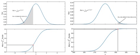
Question 1) For this problem, we will re-work homework 2a using the integrate.gauss function of scipy.integrate rather than the Simpson method to find:

P(x<1|N(0,1)): probability x<1 given a normal distribution of x with μ=0, σ=1
P(x>μ+2σ|N(175, 3))

Rather than printing your findings to the console, we will use matplotlib.pyplotto produce nicely formatted plots such as shown below. Additional requirements are:
• You should put your main function in a file called HW4a.py and all other functions in a file called NumMethods.py.
• You should import your methods from NumMethods.py with the statement:
import NumMethods as nm in your HW4a file.
• You should use numpy arrays for all of your work on this problem where arrays are needed.

Note: code stems for HW4a.py and NumMethods.py are available for download.

Question 2) Write a program that demonstrates the Least Squares Curve Fitting method. You must write and call at least the following 3 functions:

def LeastSquares(x, y, power): #calculates and returns an array containing the coefficients of the least squares polynomial.

def PlotLeastSquares(x, y, power, showpoints=True, npoints=500): #calls LeastSquares, generates data points and plots the least squares curve. If showpoints is True, also put the original data on the same plot.

def main():

A main program that uses the data given below to:
1. Call LeastSquares to generate and print the coefficients of a Linear fit.
2. Call PlotLeastSquares to display a plot for the Linear fit
3. Call LeastSquares to generate and print the coefficients of a Cubic fit.
4. Call PlotLeastSqares to display a plot for the Cubic fit
5. Uses the results from 1 and 3 to plot the datapoints, the Linear fit and the Cubic fit, all on one graph. Use proper titles, labels and legends.

x=[0.05, 0.11, 0.15, 0.31, 0.46, 0.52, 0.70, 0.74, 0.82, 0.98, 1.17]
y=[0.956, 1.09, 1.332, 0.717, 0.771, 0.539, 0.378, 0.370, 0.306, 0.242, 0.104]

Note: a code stem for HW4b.py has been written and made available.
 
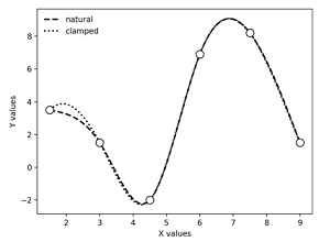
Question 3) Write a program that demonstrates the Cubic Spline Curve Fitting method. Youmust write and call at least the following 3 functions:

def CubicSpline(x, y, slope1=0, slope2=0): #calculates and returns a matrix containing the coefficients of the cubic splines. slope1 and slope2 are the slopes at the first and last points.

def PlotCubicSpline(x, y, slope1, slope2, showpoints=True, npoints=500): #calls CubicSpline, generates data points and plots the cubic spline curve. If showpoints is True, also put the original data on the same plot.

def main():

A main program that uses the data and slopes given below to:
1. Call CubicSpline to generate and print the coefficients.
2. Call PlotCubicSpline to display a plot of the natural and clamped cubic splines as shown below.

x=np.array([1.5, 3, 4.5, 6, 7.5, 9])
y=np.array([3.5, 1.5, -2, 6.9, 8.2 ,1.5])
slope1=2
slope2=-4

Notes: a code stem for HW4c.py has been made available. For a reminder of cubic spline interpolation, see the NumericalMethodsTutorial.docx.

Attachment:- SP21.rar