Reference no: EM132385029

Assignment

Topic- Numerical Linear Algebra (MATLAB)

It aims to develop your skills in programming in MATLAB, to deepen your understanding of numerical linear algebra and to explore applications of numerical linear algebra. Your solutions to this assignment will be MATLAB program listings and relevant output, together with any other mathematical derivations, notes or explanations that aids understanding.

In marking the assignment, the following criteria will be applied:

- correctness of the programs and mathemetical calculations

- clear and concise documentation, in the form of comments in the code, as to the approach being used, and

- relevance of the output in verifying the correctness of the program and in illustrating the solution.

- Some consideration will also be given to the ef?ciency of the solution.

Question 1

There is a signal b collected at M sampling points(b(1), b(2), ...b(m), ...,b(M)), and you are asked to strategically place N components x (x(1), x(2), ...,x(n),...x(N)) into the system to modify the signal profile. The modified signal profile B=Ax+b will satisfy the following condition (|??#????|) / ???? ≤∈, where B0 is the mean value of signal B. And ∈ (??) = 0.0001, ??=1,2,...M. In addition, b, B are both positive vectors. The range of components x: 0≤x(n) ≤0.006, n=1,2,...,N.

You are asked to implement the following tasks:

- Write a matlab code to minimise the 1-norm of vector x.

Note: please consider the function linprog() in matlab; The matrix A and vector b are stored in files: A.mat and b.mat, and in matlab, you can access the data as follows: Load A; load b.

- Convert the vector b to be a two-dimensional (2D) matrix data, b2d, whose size is 24X24. If you treat b2d as an image, please use low rank approximation (r=4) to implement image compression. Please plot the original image (b2d) and compressed image, and calculate the compression rate.

Note: in matlab, you can use the following code to implement data conversion:

b2d=reshape(b, [24,24]); and for image plotting, please consider function imagesc().

Question 2: Circle Centre Estimation

The accurate fitting of a circle to noisy measurements of points on its circumference is an important and much-studied problem in statistics. It has applications in many areas of research including archeology, geodesy, microwave engineering, computer vision and metrology. In this question, you will implement a least-squares algorithm for the estimation of circle centre and radius.

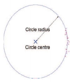
Figure 2: Noisy measurements of points on the circumference of a circular arc for Question 2.

Figure 2 illustrates the model for the data. The data are assumed to consist of N points, (x_i, y_i), i = 1 N, each slightly displaced from the circumference of a circle by noise so that

x_i = a + r cosθ_i + ξ_i,

y_i= b + r sinθ_i +η_i.

Here, (a ,b) is the centre of the circle, r is its radius, the θ_i are the angles along the arc on which the points lie and the ξ_i and η_i are noise.

Given the (x_i, y_i), it is possible to formulate the problem of estimating (a, b) as a linear least squares problem. First of all, define the function

r_i(a,b) = √(x_i - a)² + (y_i - b)²,

i.e., the distance from the centre to the ith noisy point on the circumference. If the centre and radius has been estimated well then r_i(a, b) should be approximately equal to r for all i = 1 ..... N. Hence, one approach to estimating a, I) and r would be to choose those values that minimise the mean square error between the r_i(a,b) and r, i.e., minimise the expression

(1/N) _i=1Σ^N[r_i(a,b) - r]² .

However, this expression is difficult to work with because of the square-root terms in each of the ri(a, b). It's much easier to minimise the expression

(1/N) _i=1Σ^N[r_i(a,b)² - r²]² .

with respect to a, b and r because the square-root terms disappear. In fact, as we will see, this transforms the problem into a linear least squares problem. Now, substitute r with c where

c = r² - a² - b².

The expression we seek to minimise can then be written as an objective function f in three variables, a, b and c, such that

ƒ (a, b,c) = _i=1Σ^N[x_i² - 2ax_i + y_i- 2by_i -c)

(Notice that we have discarded the constant 1/N term.) If we write the parameters to be estimated in a vector
v= (abc)

then we can rewrite the objective function as

ƒ (v) = ||Mv -w||²                 (1)

for constant matrix M and vector w. This is a linear least squares problem and we know from Lecture LA09 that ƒ(v) is minimised when

v = M⁺w

(a) Derive expressions for the matrix M and the vector w in (1).

(b) Write a MATLAB function to estimate circle centre and radius from a matrix P containing the coordinates (x_i, y_i) as columns.

(c) Generate a plot similar to Figure 2. To do this, choose the true value of r to be around 20, set the Og to be equally spaced over an arc of around 90° and use MATLAB'S randn function to create the noise components (ξ_i , η_i) . Plot the noisy points, the true centre and the estimated centre, the true circle and the estimated one.