Reference no: EM132495864
Time Series Analysis
Problem 1:
With the gasoline time series data from the given table, show the exponential smoothing forecasts using α = 0.1.
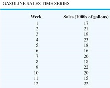
a. Applying the MSE measure of forecast accuracy, would you prefer a smoothing constant of α = 0.1 or α = 0.2 for the gasoline sales time series? Do not round your interim computations and round your final answers to three decimal places.
b. α = 0.1 α = 0.2
MSE
c.
Prefer: ------
d. Are the results the same if you apply MAE as the measure of accuracy? Do not round your interim computations and round your final answers to three decimal places.
e. α = 0.1 α = 0.2
MAE
f.
Prefer: -------
g. What are the results if MAPE is used? Do not round your interim computations and round your final answers to two decimal places.
h. α = 0.1 α = 0.2
MAPE %
%
i.
Prefer:------------
Problem 2:
Consider the following time series.
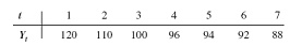
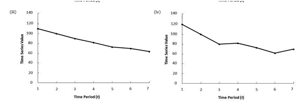
a. Choose the correct time series plot.
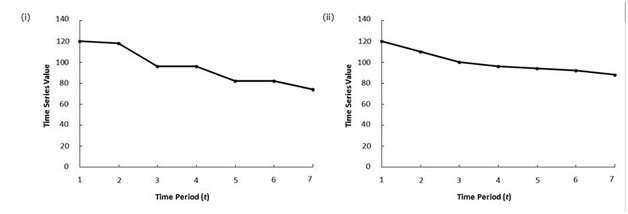
(i) (ii)
(iii) (iv)
b.
-------------
c.
d.
e.
f.
g.
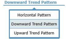
What type of pattern exists in the data?
---------------which one from bottom options
h. Use simple linear regression analysis to find the parameters for the line that minimizes MSE for this time series. Do not round your interim computations and round your final answers to three decimal places. For subtractive or negative numbers use a minus sign. (Example: -300)
y-intercept, b0 =
Slope, b1 =
MSE =
i. C What is the forecast for t = 8? If required, round your answer to three decimal places.