Reference no: EM132245196
Applied Statistics Assignment Problems set -
Q1. Suppose a least-squares regression line is given by y^ = 4.302x - 3.293. What is the mean value of the response variable if x = 20?
Q2. If H0: β1 = 0 is not rejected, what is the best estimate for the value of the response variable for any value of the explanatory variable?
Choose the correct answer below.
A. The best estimate is the value of the response variable for the data point closest to the particular value of the explanatory variable. If there is more than one data point at that value, it is the mean of the response variables at that point.
B. There is no way to estimate the value of the response variable.
C. The best estimate is the mode of the sample y values.
D. The best estimate is the sample mean of y.
Q3. For the data set shown below, complete parts (a) through (d) below.
|
x
|
3
|
4
|
5
|
7
|
8
|
|
y
|
5
|
7
|
8
|
12
|
15
|
(a) Find the estimates of β0 and β1.
(b) Compute the standard error, the point estimate for σ.
(c) Assuming the residuals are normally distributed, determine sb_1.
(d) Assuming the residuals are normally distributed, test H0: β1 = 0 versus H1: β1 ≠ 0 at the α = 0.05 level of significance. Use the P-value approach.
The P-value for this test is _______. (Round to three decimal places as needed.)
Make a statement regarding the null hypothesis and draw a conclusion for this test. Choose the correct answer below.
A. Reject H0. There is sufficient evidence at the α = 0.05 level of significance to conclude that a linear relation exists between x and y.
B. Reject H0. There is not sufficient evidence at the α = 0.05 level of significance to conclude that a linear relation exists between x and y.
C. Do not reject H0. There is not sufficient evidence at the α = 0.05 level of significance to conclude that a linear relation exists between x and y.
D. Do not reject H0. There is sufficient evidence at the α = 0.05 level of significance to conclude that a linear relation exists between x and y.
Q4. For the data set shown below, complete parts (a) through (d) below.
|
x
|
20
|
30
|
40
|
50
|
60
|
|
y
|
100
|
93
|
91
|
85
|
68
|
(a) Use technology to find the estimates of β0 and β1.
(b) Use technology to compute the standard error, the point estimate for σ.
(c) Assuming the residuals are normally distributed, use technology to determine sb_1.
(d) Assuming the residuals are normally distributed, test H0: β1 = 0 versus H1: β1 ≠ 0 at the α = 0.05 level of significance. Use the P-value approach.
Determine the P-value for this hypothesis test.
Which of the following conclusions is correct?
A. Do not reject H0 and conclude that a linear relation does not exist between x and y.
B. Reject H0 and conclude that a linear relation does not exist between x and y.
C. Reject H0 and conclude that a linear relation exists between x and y.
D. Do not reject H0 and conclude that a linear relation exists between x and y.
Q5. A pediatrician wants to determine the relation that may exist between a child's height and head circumference. She randomly selects 5 children and measures their height and head circumference. The data are summarized below. Complete parts (a) through (f) below.
|
Height (inches), x
|
26.5
|
25.5
|
27.75
|
27.5
|
27
|
|
Head Circumference (inches), y
|
17.3
|
17.1
|
17.6
|
17.5
|
17.5
|
(a) Treating height as the explanatory variable, x, use technology to determine the estimates of β0 and β1.
(b) Use technology to compute the standard error of the estimate, se.
(c) A normal probability plot suggests that the residuals are normally distributed. Use technology to determine sb_1.
(d) A normal probability plot suggests that the residuals are normally distributed. Test whether a linear relation exists between height and head circumference at the α = 0.01 level of significance. State the null and alternative hypotheses for this test.
Choose the correct answer below.
A. H0: β0 = 0
H1: β0 ≠ 0
B. H0: β0 = 0
H1: β0 > 0
C. H0: β1 = 0
H1: β1 > 0
D. H0: β1 = 0
H1: β1 ≠ 0
Determine the P-value for this hypothesis test.
What is the conclusion that can be drawn?
A. Reject H0 and conclude that a linear relation exists between a child's height and head circumference at the level of significance α = 0.01.
B. Do not reject H0 and conclude that a linear relation does not exist between a child's height and head circumference at the level of significance α = 0.01.
C. Reject H0 and conclude that a linear relation does not exist between a child's height and head circumference at the level of significance α = 0.01.
D. Do not reject H0 and conclude that a linear relation exists between a child's height and head circumference at the level of significance α = 0.01.
(e) Use technology to construct a 95% confidence interval about the slope of the true least-squares regression line.
Lower bound:
Upper bound:
(f) Suppose a child has a height of 26.5 inches. What would be a good guess for the child's head circumference?
Q6. As concrete cures, it gains strength. The following data represent the 7-day and 28-day strength in pounds per square inch (psi) of a certain type of concrete. Complete parts (a) through (f) below.
|
7-Day Strength (psi), x
|
3340
|
3380
|
2300
|
2890
|
3330
|
|
28-Day Strength (psi), y
|
4630
|
5020
|
4070
|
4620
|
4850
|
(a) Treating the 7-day strength as the explanatory variable, x, use technology to determine the estimates of β0 and β1.
(b) Compute the standard error of the estimate, se.
(c) A normal probability plot suggests that the residuals are normally distributed. Determine sb_1. Use the answer from part (b).
(d) A normal probability plot suggests that the residuals are normally distributed. Test whether a linear relation exists between 7-day strength and 28-day strength at the α = 0.05 level of significance.
State the null and alternative hypotheses. Choose the correct answer below.
A. H0: β0 = 0
H1: β0 ≠ 0
B. H0: β1 = 0
H1: β1 ≠ 0
C. H0: β1 = 0
H1: β0 > 0
D. H0: β1 = 0
H1: β1 > 0
Determine the P-value of this hypothesis test.
What is the conclusion that can be drawn?
A. Reject H0 and conclude that a linear relation does not exist between the 7-day and 28-day strength of a certain type of concrete at the α = 0.05 level of significance.
B. Reject H0 and conclude that a linear relation exists between the 7-day and 28-day strength of a certain type of concrete at the α = 0.05 level of significance.
C. Do not reject H0 and conclude that a linear relation exists between the 7-day and 28-day strength of a certain type of concrete at the α = 0.05 level of significance.
D. Do not reject H0 and conclude that a linear relation does not exist between the 7-day and 28-day strength of a certain type of concrete at the α = 0.05 level of significance.
(e) Construct a 95% confidence interval about the slope of the true least-squares regression line.
Lower bound:
Upper bound:
(f) What is the estimated mean 28-day strength of this concrete if the 7-day strength is 3000 psi?
Q7. A doctor wanted to determine whether there is a relation between a male's age and his HDL (so-called good) cholesterol. The doctor randomly selected 17 of his patients and determined their HDL cholesterol. The data obtained by the doctor is the in the data table below.
Age vs. HDL Cholesterol data
|
Age, x
|
HDL Cholesterol, y
|
Age, x
|
HDL Cholesterol, y
|
|
38
|
58
|
39
|
45
|
|
41
|
54
|
66
|
61
|
|
44
|
32
|
32
|
55
|
|
34
|
55
|
50
|
34
|
|
54
|
33
|
27
|
43
|
|
53
|
41
|
54
|
37
|
|
62
|
40
|
50
|
53
|
|
59
|
40
|
38
|
28
|
|
28
|
46
|
|
|
Complete parts (a) through (f) below.
(a) Draw a scatter diagram of the data, treating age as the explanatory variable. What type of relation, if any, appears to exist between age and HDL cholesterol?
A. The relation appears to be nonlinear.
B. The relation appears to be linear.
C. There does not appear to be a relation.
(b) Determine the least-squares regression equation from the sample data.
y^ = ______ x+ _____
(c) Are there any outliers or influential observations?
No
Yes
(d) Assuming the residuals are normally distributed, test whether a linear relation exists between age and HDL cholesterol levels at the α = 0.01 level of significance.
What are the null and alternative hypotheses?
A. H0: β1 =0; H1: β1 ≠ 0
B. H0: β1 = 0; H1: β1 > 0
C. H0: β1 = 0; H1: β1 < 0
Use technology to compute the P-value. Use the Tech Help button for further assistance.
What conclusion can be drawn at a = 0.01 level of significance?
A. Reject the null hypothesis because the P-value is less than α = 0.01.
B. Do not reject the null hypothesis because the P-value is greater than α = 0.01.
C. Do not reject the null hypothesis because the P-value is less than α = 0.01.
D. Reject the null hypothesis because the P-value is greater than α = 0.01.
(e) Assuming the residuals are normally distributed, construct a 95% confidence interval about the slope of the true least-squares regression line.
Lower Bound =
Upper Bound =
(f) For a 42-year-old male patient who visits the doctor's office, would using the least-squares regression line obtained in part (b) to predict the HDL cholesterol of this patient be recommended?
If the null hypothesis was rejected, that means that this least-squares regression line can accurately predict the HDL cholesterol of a patient. If the null hypothesis was not rejected, that means the least-squares regression line cannot accurately predict the HDL cholesterol of a patient.
Should this least-squares regression line be used to predict the patient's HDL cholesterol? Choose the correct answer below.
A. No, because the null hypothesis was not rejected.
B. Yes, because the null hypothesis was not rejected.
C. Yes, because the null hypothesis was rejected.
D. No, because the null hypothesis was rejected.
A good estimate for the HDL cholesterol of this patient is _____ (Round to two decimal places as needed.)
Q8. The data in the accompanying table represent the population of a certain country every 10 years for the years 1900-2000. An ecologist is interested in finding an equation that describes the population of the country over time.
Population
|
Year, x
|
Population, y
|
Year, x
|
Population, y
|
|
1900
|
76,212
|
1960
|
179,323
|
|
1910
|
92,228
|
1970
|
203,302
|
|
1920
|
106,021
|
1980
|
226,542
|
|
1930
|
123,202
|
1990
|
248,709
|
|
1940
|
132,164
|
2000
|
281,421
|
|
1950
|
151,325
|
|
|
Complete parts (a) through (f) below.
(a) Determine the least-squares regression equation, treating year as the explanatory variable. Choose the correct answer below.
A. y^ = 1,236,370x - 3,771,539
B. y^ = 2,019x - 3,771,539
C. y^ = 2,019X - 1,537,083
D. y^ = - 3,771,539x + 2,019
(b) A normal probability plot of the residuals indicates that the residuals are approximately normally distributed. Test whether a linear relation exists between year and population. Use the α = 0.01 level of significance.
State the null and alternative hypotheses. Choose the correct answer below.
A. H0: β1 = 0
H1: β1 > 0
B. H0: β0 = 0
H1: β0 ≠ 0
C. H0: β0 = 1
H1: β0 > 0
D. H0: β1= 0
H1: β1 ≠ 0
Determine the P-value of this hypothesis test.
State the appropriate conclusion. Choose the correct answer below.
A. Reject H0. There is sufficient evidence to conclude that a linear relation exists between year and population.
B. Do not reject H0. There is sufficient evidence to conclude that a linear relation exists between year and population.
C. Reject H0. There is not sufficient evidence to conclude that a linear relation exists between year and population.
D. Do not reject H0. There is not sufficient evidence to conclude that a linear relation exists between year and population.
(c) Draw a scatter diagram, treating year as the explanatory variable.
(d) Plot the residuals against the explanatory variable, year. Choose the correct graph below.
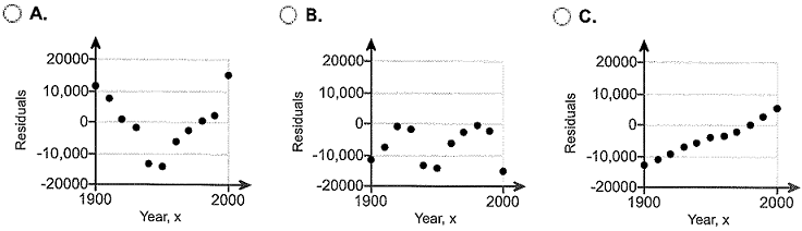
(e) Does a linear model seem appropriate based on the scatter diagram and residual plot?
Yes
No
(f) What is the moral?
A. The moral is that explanatory variables may indicate that a linear relation between the two variables does not exist even though diagnostic tools (such as residual plots) indicate that a linear model is appropriate.
B. The moral is that inferential procedures may indicate that a linear relation between the two variables exists even though diagnostic tools (such as residual plots) indicate that a linear model is inappropriate.
C. The moral is that inferential procedures may indicate that a nonlinear relation between the two variables exists even though diagnostic tools (such as residual plots) indicate that a linear model is appropriate.
Q9. The accompanying data represent the total compensation for 12 randomly selected chief executive officers (CEOs) and the company's stock performance. Use the data to complete parts (a) through (d).
Data Table of Compensation and Stock Performance
|
Company
|
Compensation (millions of dollars)
|
Stock Return (%)
|
|
A
|
14.26
|
72.11
|
|
B
|
3.69
|
63.23
|
|
C
|
7.88
|
149.68
|
|
D
|
1.04
|
30.85
|
|
E
|
1.83
|
10.08
|
|
F
|
2.16
|
29.06
|
|
G
|
12.87
|
0.64
|
|
H
|
7.36
|
68.11
|
|
I
|
9.93
|
58.96
|
|
J
|
3.33
|
50.21
|
|
K
|
21.79
|
27.04
|
|
L
|
5.21
|
30.44
|
(a) Treating compensation as the explanatory variable, x, use technology to determine the estimates of β0 and β1.
(b) Assuming that the residuals are normally distributed, test whether a linear relation exists between compensation and stock return at the α = 0.01 level of significance.
What are the null and alternative hypotheses?
A. H0: β1 ≠ 0
H1: β1 = 0
B. H0: β1 = 0
H1: β1 ≠ 0
C. H0: β0 ≠ 0
H1: β0 = 0
D. H0: β0 = 0
H1: β0 ≠ 0
Compute the test statistic using technology.
Compute the P-value using technology.
State the appropriate conclusion. Choose the correct answer below.
A. Reject H0. There is sufficient evidence to conclude that a linear relation exists between compensation and stock return.
B. Do not reject H0. There is sufficient evidence to conclude that a linear relation exists between compensation and stock return.
C. Reject H0. There is not sufficient evidence to conclude that a linear relation exists between compensation and stock return.
D. Do not reject H0. There is not sufficient evidence to conclude that a linear relation exists between compensation and stock return.
(c) Assuming the residuals are normally distributed, construct a 99% confidence interval for the slope of the true least-squares regression line.
Lower bound =
Upper bound =
(d) Based on your results to parts (b) and (c), would you recommend using the least-squares regression line to predict the stock return of a company based on the CEO's compensation? Why? What would be a good estimate of the stock return based on the data in the table?
A. The regression line could be used to predict the stock return. The test in part (b) and the confidence interval in part (c) both confirm that there is a relationship between the variables.
B. Based on the results from parts (b), the regression line should not be used to predict the stock return. However, the results from part (c) indicate that the regression line should be used. The results are not conclusive and further analysis of the data is needed.
C. Based on the results from parts (b), the regression line could be used to predict the stock return. However, the results from part (b) indicate that the regression line should not be used. The results are not conclusive and further analysis of the data is needed.
D. Based on the results from parts (b) and (c), the regression line should not be used to predict the stock return. The mean stock return would be a good estimate of the stock return based on the data in the table.
Q10. The data in the accompanying table represent the population of a certain country every 10 years for the years 1900-2000. An ecologist is interested in finding an equation that describes the population of the country over time.
Population
|
Year, x
|
Population, y
|
Year, x
|
Population, y
|
|
1900
|
76,212
|
1960
|
179,323
|
|
1910
|
92,228
|
1970
|
203,302
|
|
1920
|
106,021
|
1980
|
226,542
|
|
1930
|
123,202
|
1990
|
248,709
|
|
1940
|
132,164
|
2000
|
281,421
|
|
1950
|
151,325
|
|
|
Complete parts (a) through (f) below.
(a) Determine the least-squares regression equation, treating year as the explanatory variable. Choose the correct answer below.
A. y^ = 2,019x - 3,771,539
B. y^ = 3,771,539x + 2,019
C. y^ = 2,019x - 1,537,083
D. y^ =1,236,370x - 3,771,539
(b) A normal probability plot of the residuals indicates that the residuals are approximately normally distributed. Test whether a linear relation exists between year and population. Use the α = 0.01 level of significance.
State the null and alternative hypotheses. Choose the correct answer below.
A. H0: β1 = 0
H1: β1≠ 0
B. H0: β0 = 0
H1: β1 > 0
C. H0: β0 = 0
H1: β0 ≠ 0
D. H0: β1 =0
H1: β1 > 0
Determine the P-value of this hypothesis test.
State the appropriate conclusion. Choose the correct answer below.
A. Do not reject H0. There is sufficient evidence to conclude that a linear relation exists between year and population.
B. Do not reject H0. There is not sufficient evidence to conclude that a linear relation exists between year and population.
C. Reject H0. There is not sufficient evidence to conclude that a linear relation exists between year and population.
D. Reject H0. There is sufficient evidence to conclude that a linear relation exists between year and population.
(c) Draw a scatter diagram, treating year as the explanatory variable.
(d) Plot the residuals against the explanatory variable, year. Choose the correct graph below.
(e) Does a linear model seem appropriate based on the scatter diagram and residual plot?
Yes
No
(f) What is the moral?
A. The moral is that inferential procedures may indicate that a linear relation between the two variables exists even though diagnostic tools (such as residual plots) indicate that a linear model is inappropriate.
B. The moral is that inferential procedures may indicate that a nonlinear relation between the two variables exists even though diagnostic tools (such as residual plots) indicate that a linear model is appropriate.
C. The moral is that explanatory variables may indicate that a linear relation between the two variables does not exist even though diagnostic tools (such as residual plots) indicate that a linear model is appropriate.