Reference no: EM132390623

Assignment

Book - OpenIntro Statistics By David Diez, Mine C ¸ etinkaya-Rundel and Christopher D Barr. (Chapter 6 Inference for categorical data and Chapter 7 Inference for numerical data.)

Chi-square tests, ANOVA, revision

Chi-square tests and ANOVA

Textbook exercises: 6.34, 6.50, 7.38, 7.46

6.34  Microhabitat factors associated with forage and bed sites of barking deer in Hainan Island, China were examined. In this region woods make up 4.8% of the land, cultivated grass plot makes up 14.7%, and deciduous forests make up 39.6%. Of the 426 sites where the deer forage, 4 were categorized as woods, 16 as cultivated grassplot, and 61 as deciduous forests. The table below summarizes these data.

(a) Write the hypotheses for testing if barking deer prefer to forage in certain habitats over others.

(b) What type of test can we use to answer this research question?

(c) Check if the assumptions and conditions required for this test are satisfied.

(d) Do these data provide convincing evidence that barking deer prefer to forage in certain habitats over others? Conduct an appropriate hypothesis test to answer this research question.

6.50 Coffee and Depression. Researchers conducted a study investigating the relationship between caffeinated coffee consumption and risk of depression in women. They collected data on 50,739 women free of depression symptoms at the start of the study in the year 1996, and these women were followed through 2006.

The researchers used questionnaires to collect data on caffeinated coffee consumption, asked each individual about physician- diagnosed depression, and also asked about the use of antidepressants. The table below shows the distribution of incidences of depression by amount of caffeinated coffee consumption.

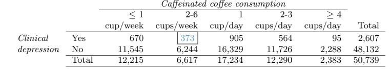
(a) What type of test is appropriate for evaluating if there is an association between coffee intake and depression?

(b) Write the hypotheses for the test you identified in part (a).

(c) Calculate the overall proportion of women who do and do not suffer from depression.

(d) Identify the expected count for the highlighted cell, and calculate the contribution of this cell to the test statistic, i.e. (Observed − Expected) 2 /Expected.

(e) The test statistic is χ

2 = 20.93. What is the p-value?

(f) What is the conclusion of the hypothesis test?

(g) One of the authors of this study was quoted on the NYTimes as saying it was “too early to recommend that women load up on extra coffee” based on just this study.53 Do you agree with this statement? Explain your reasoning.

7.38 Teaching descriptive statistics.

A study compared five different methods for teaching descriptive statistics. The five methods were traditional lecture and discussion, programmed textbook instruction, programmed text with lectures, computer instruction, and computer instruction with lectures. 45 students
were randomly assigned, 9 to each method. After completing the course, students took a 1-hour exam.

(a) What are the hypotheses for evaluating if the average test scores are different for the different teaching methods?

(b) What are the degrees of freedom associated with the F-test for evaluating these hypotheses?

(c) Suppose the p-value for this test is 0.0168. What is the conclusion?

7.46 True / False: ANOVA, Part II.

Determine if the following statements are true or false, and explain your reasoning for statements you identify as false.

If the null hypothesis that the means of four groups are all the same is rejected using ANOVA at a 5% significance level, then ...

(a) we can then conclude that all the means are different from one another.

(b) the standardized variability between groups is higher than the standardized variability within groups.

(c) the pairwise analysis will identify at least one pair of means that are significantly different.

(d) the appropriate α to be used in pairwise comparisons is 0.05 / 4 = 0.0125 since there are four groups.

Revision Textbook exercises: 6.16, 7.5, 7.6, 7.12, 7.20(c),(e),(g), 7.32

6.16 Legalize Marijuana, Part II. As discussed in Exercise 6.10, the General Social Survey reported a sample where about 61% of US residents thought marijuana should be made legal. If we wanted to limit the margin of error of a 95% confidence interval to 2%, about how many Americans would we need to survey?

7.5 Working backwards, Part I. A 95% confidence interval for a population mean, μ, is given as (18.985, 21.015). This confidence interval is based on a simple random sample of 36 observations. Calculate the sample mean and standard deviation. Assume that all conditions  necessary for inference are satisfied. Use the t-distribution in any calculations.

7.6 Working backwards, Part II. A 90% confidence interval for a population mean is (65, 77). The population distribution is approximately normal and the population standard deviation is unknown. This confidence interval is based on a simple random sample of 25 observations. Calculate the sample mean, the margin of error, and the sample standard deviation.

7.12 Auto exhaust and lead exposure. Researchers interested in lead exposure due to car exhaust sampled the blood of 52 police officers subjected to constant inhalation of automobile exhaust fumes while working traffic enforcement in a primarily urban environment. The blood samples of these officers had an average lead concentration of 124.32 μg/l and a SD of 37.74 μg/l; a previous study of individuals from a nearby suburb, with no history of exposure, found an average blood level concentration of 35 μg/l.9

(a) Write down the hypotheses that would be appropriate for testing if the police officers appear to have been exposed to a different concentration of lead.

(b) Explicitly state and check all conditions necessary for inference on these data.

(c) Regardless of your answers in part (b), test the hypothesis that the downtown police officers have a higher lead exposure than the group in the previous study. Interpret your results in context.

7.20 High School and Beyond, Part I. The National Center of Education Statistics conducted a survey of high school seniors, collecting test data on reading, writing, and several other subjects. Here we examine a simple random sample of 200 students from this survey. Side-by-side box plots of reading and writing scores as well as a histogram of the differences in scores are shown below.

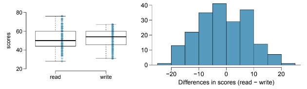
(c) Create hypotheses appropriate for the following research question: is there an evident difference in the average scores of students in the reading and writing exam?

(e) The average observed difference in scores is  ¯xread−write = −0.545, and the standard deviation of the differences is 8.887 points. Do these data provide convincing evidence of a difference between the average scores on the two exams?

(g) Based on the results of this hypothesis test, would you expect a confidence interval for the average difference between the reading and writing scores to include 0? Explain your reasoning.

7.32 True / False: comparing means. Determine if the following statements are true or false, and explain your reasoning for statements you identify as false.

(a) When comparing means of two samples where n1 = 20 and n2 = 40, we can use the normal model for the difference in means since n2 ≥ 30.

(b) As the degrees of freedom increases, the t-distribution approaches normality.

(c) We use a pooled standard error for calculating the standard error of the difference between means when sample sizes of groups are equal to each other.