Reference no: EM132311575

Learning Outcomes -

a. Develop and implement signal processing algorithms in Matlab
b. Undertake in-depth design of digital filters

Assessment

Introduction

The objective of this assessment is for each student to demonstrate understanding of the contents of lecture materials in the unit by applying the principles and concepts in lecture notes. Concepts covered by this assignment include z-transforms, and FIR filter design.

Section 1. FIR filter design

In general, we have 3 commonly used FIR filter design techniques

(1) Windowed Fourier series approach
(2) Frequency sampling approach
(3) Computer-based optimization methods

In this assignment we practice the first and the second methods in designing FIR filters

Designing a low pass FIR filter using Windowed Fourier Series approach

The amplitude frequency response of an ideal low pass filter is shown in Figure. 1. Its impulse response can be found from its inverse Fourier transform as:

Figure 1. Ideal low pass filter amplitude frequency response (left) and impulse response (right)

Using the equation (1) we can find all the impulse response samples. The filter is IIR but by truncating the impulse response to a limited number of samples we can make it an FIR filter. To do so we usually select M samples (M is usually odd number) around n=0 as shown in Figure 2.

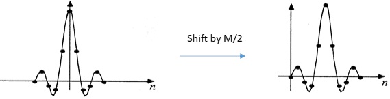
Figure 2. Truncated impulse response

By multiplying the resultant impulse response by a window we can reduce unwanted ripples in the spectrum.

The following Matlab code designs a FIR filter with Windowed Fourier Series approach.

wp=pi/8; % lowpass filter bandwidth
M=121;
n=-(M-1)/2:(M-1)/2; % selection time window
h0=(wp/pi)*sinc((wp/pi)*n); % truncated impulse response
h=h0.*rectwin(M)'; % windowing
% h=h0.*hamming(M)';% windowing
% h=h0.*hanning(M)';% windowing
% h=h0.*bartlett(M)';% windowing
% h=h0.*blackman(M)';% windowing
figure;plot(h)
ylabel('Impulse response')
xlabel('Samples')

% spectrum
FFTsize=512;
pxx=20*log10(abs(fft(h,FFTsize)));
fxx=(0:(FFTsize/2)-1)*(pi/(FFTsize/2));
figure;plot(fxx,pxx(1:FFTsize/2));
ylabel('Amplitude[dB]');
xlabel('frequency [Radian]');grid on

Do the following tasks and plot all the graphs in your report:

1) Run the above program and plot the impulse response and the amplitude spectrum of the filter.

2) Measure the filter frequency response at ωp = pi/8. Is it close to the expected value of -6dB? How much is the maximum ripple in the pass band.

3) This filtering technique does not define any cutoff. If we assume the stopband starts at -20dB, measure the ratio of the transient band to the pass band.

4) Increase the filter impulse response length to M = 255 and run the program.

a) If we assume the stopband starts at -20dB, measure the ratio of the transient band to the passband.
b) Measure the ripple in the passbad.
c) Discuss the effect of the filter length on the ripples and stopband attenuation.

5) Use Hamming and Hanning window with the filter impulse response length, M=121, and discuss the effect of the window on the ripples and stopband attenuation.

6) Change ωp=pi/4 and repeat 1) and discuss the effect.

1 -2 Designing a bandpass FIR filter using Windowed Fourier Series approach

A FIR lowpass filter can be converted to a bandpass filter by multiplying its impulse response by a complex sinusoidal with the frequency of the center frequency of the desired bandpass filter. In fact, the whole filter band shifts by this frequency. The following MATLAB code designs such a bandpass filter:

wp=pi/16; % lowpass filter bandwidth M=121;
n=-(M-1)/2:(M-1)/2; % selection time window h0=(wp/pi)*sinc((wp/pi)*n); % truncated impulse response h1=h0.*rectwin(M)'; % windowing
w0=pi/4; % BPF center frequency
h=h1.*exp(j*w0*n); % Lowpass to bandpass conversion

figure;
subplot(211);plot(real(h));ylabel('Real part of impulse response') xlabel('samples')
subplot(212);plot(imag(h));ylabel('imag part of impulse response') xlabel('samples')
% spectrum FFTsize=512;
pxx=20*log10(abs(fft(h,FFTsize))); fxx=(0:(FFTsize/2)-1)*(pi/(FFTsize/2)); figure;plot(fxx,pxx(1:FFTsize/2));ylabel('Amplitude [dB]');xlabel('frequency [Radian]');grid on

Do the following tasks and plot all the graphs in your report:

7) Run the above program and plot the impulse response and the amplitude spectrum of the filter.

8) What are the passband edges ωp1 ωp2. Measure the attenuation in frequency response at these frequencies and compare them with the expected value of -6dB.

9) Measure the maximum ripple in the passband.

10) Increase ωp to pi/4 and discuss the result

1 -3 Designing a band-stop FIR filter using Frequency sampling approach

In this section, you must write your own code to design a band stop filter using the knowledge you gained from the sections 1-1 and 1-2

Write a code to design a band-stop filter. Design a band-stop filter by having the following block diagram in your mind

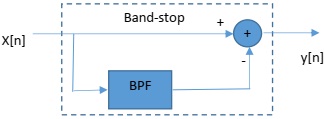
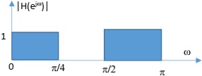
The spectrum mask is as the following:

11) Report your MATLAB code. Select the filter impulse response length M=121;

12) Plot the frequency response, |H(ej^ω)|, of your filter on the top of the spectrum mask in a single plot.

13) Plot 20*log10(|H(ej^ω)|) of your filter on the top of the spectrum mask in dB in a single plot.

14) Measure the amplitude at ω = [Π/4, 3Π/4, Π/2] on your second plot.

15) Find the deepest point in your frequency response in dB. How you can increase the depth of the stopband?

1-4 Designing a low pass FIR filter using Frequency sampling approach

In the frequency sampling approach, we design an amplitude response in the frequency domain and find the impulse response by applying IFFT on that frequency response.

The following MATLAB code designs a low pass FIR filter using Frequency sampling approach. It initially designs the amplitude spectrum and the apply IFFT. Using some shifts it finds the truncated impulse response.

wp=pi/8;
M=121;
FFTsize=512;
% passband frequency samples
Np=fix((wp/(2*pi))*FFTsize); % number of pass band samples
Ns=FFTsize/2-Np; % number of stop band samples
H1=[ones(1,Np) zeros(1,Ns+1)];
H=[H1 H1(end:-1:2)]; % sampled frequency spectrum;
fxx=(0:(FFTsize/2)-1)*(pi/(FFTsize/2));
figure;plot(fxx,H(1:FFTsize/2));
ylabel('Amplitude');
xlabel('frequency [Radian]');grid on

% finding impulse response by truncating
h1=real(ifft(H));
h0=[ h1(end-(M-1)/2+1:end) h1(1:1+(M-1)/2)];
figure;plot(h0)
ylabel('Impulse response')
xlabel('Samples')
% spectrum
pxx=20*log10(abs(fft(h0,FFTsize)));
fh=figure;plot(fxx,pxx(1:FFTsize/2));hold on;
% effect of windowing
h=h0.*hanning(M)';% windowing
% spectrum
pxx=20*log10(abs(fft(h,FFTsize)));
figure(fh);plot(fxx,pxx(1:FFTsize/2));grid on;
legend('rectwin','hanning')

Do the following tasks and plot all the graphs in your report:

16) Run the above program and plot the impulse response and the amplitude spectrum of the filter. Try to understand what the program does.

17) Use the above program as your base, design a band pass filter that passes the frequencies between pi/8<w<pi/4. Only modify the lines 5-7 and do not touch the rest of the program.

Section 2. Analyzing a system in Z and time domain

A digital system is given by the following transfer function:

H(z) = 1 - 0.2z^-1/(1 - 0.5z^-1)(1 - 0.3z^-1)

18) Assume the system is causal. Draw its region of convergence (ROC) in the z-plane

19) Is the system stable or unstable? Why?

20) Determine the system difference equation in the form of

∑_k=0^N a_kY[n-k] = ∑_k=0^M b_kx[n-k]

21) Give the values for ai and bj , N and M

22) Sketch the magnitude of the frequency response of the system between 0 and Π

23) Suppose the above transfer function is a filter, what type of filter is it? (a low-pass, high-pass, band-pass, band-stop or all-pass)

24) Sketch a block diagram for implementing this system

25) Find the system causal impulse response (use partial fraction decomposition of the equation (1) )

26) Assume the initial condition is zero, enter a unit impulse to the system and find the impulse response of the system h[n] for the first 10 samples and compare it with the step11

Section 3. Filtering

Use the filter impulse response "h" you found by running the given program in the section 1-3 with a Hanning window.

Run the following code

x=randn(1,5000); % signal to be filtered
NFFT=512; % FFTT size (N)
overlap samples=0; % number of overlap samples in time frames
y=conv(x,h); % filtering operation using convolution
[Pxx,W] = pwelch(y,hamming(NFFT),overlap_samples,NFFT);
figure;plot(W,Pxx);xlabel('W [radian] from 0-pi');ylable(' power spectral
density')

27) Plot and include the plot in your report. Simply, mention the application of the "pwelch" program, and what are its input parameters.

Run the following Matlab code
x=[-zeros(1,500) ones(1,1000) zeros(1,500)]; % signal to be filtered
y=conv(x,h); % filtering operation using convolution
figure;plot(x,'.-')
hold on;plot(y,'.-'); grid;
xlabel('sample')
legend('filter input signal','filter output')

28) Measure the filter delay and find a ratio of the filter delay to the filter impulse response length

Attachment:- Digital Signal Processing.rar