Reference no: EM13748546

1. Suppose that the true relationship between high school graduation rates, school funding, population density, and construction wages for all counties in the United States is given by

hsgrad = β₀ + β₁sfunding + β₂popdensity + β₃cwage + u,

and suppose that, miraculously, E(u|sfunding, popdensity, cwage) = 0.

(a) Suppose the sample only includes urban counties (counties with popdensity > 10). Would OLS produce an unbiased estimate of β1? Why or why not?

(b) Suppose the sample only includes urban counties (counties with popdensity > 10). Would OLS produce an unbiased estimate of β2? Why or why not?

(c) Suppose the sample only includes counties where hsgrad < .90. Would OLS produce an unbiased estimate of β1? Why or why not?

(d) Suppose the sample only includes counties where hsgrad < .90. Would OLS produce an unbiased estimate of β2? Why or why not?

2. Consider the regression model of

murderratet = β₀ + β₁ policebudget_t + ε_t

where murderratet is the annual murder rate in Bakersfield in year t, policebudgett is the annual police budget in Bakersfield. The data set available has one observation for each of the last 40 years.

(a) What assumptions must hold for OLS to give an unbiased estimate of β₁, the structural effect of increasing the police budget on the murder rate?

(b) Which, if any, of these assumptions are violated if policebudgett depends on murderrate_t-1?

(c) What assumptions must hold for OLS to give an consistent estimate of the β₁, structural effect of increasing the police budget on the murder rate?

(d) Which, if any, of these assumptions are violated if policebudgett depends on murderrate_t-1?

3. Let yct be the labor force participation rate of married, non-Hispanic females in city c in year t.

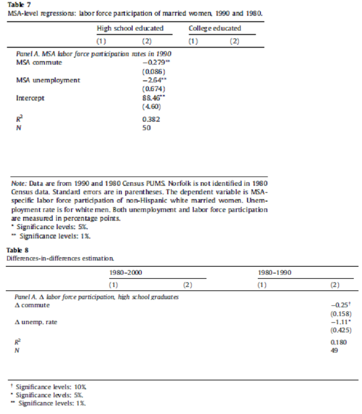
Let commutect be the average commute time in year t and city c and let unempct be the male unemployment rate in year t and city c. Table 7 from Black, Kolesnikova, and Taylor (2014) at the end of the exam shows the results of running Ordinary Least Square using a cross-section (with t=1990) for the regression model

y_ct = β₀ + β_commute · commute_ct + β_unemp · unemp_ct + u_ct.

Table 8 shows the results a regression model that uses differences in the 1980 and 1990 observations for each city,

?_yc = β_commute · ?commute_c + β_unemp · ?unempc + ?u_c.

(a) Let ct be a random, idiosyncratic effect that is uncorrelated with everything. Let ξc be a city-specific effect that is correlated with commute times and unemployment but that is constant over time. (One could think of ξc being an omitted variable that measures local traditions of good governance, for example.) Suppose the error term uct is a combination of both effects, uct = ξc + ct. Are the results of cross section OLS regression reported in table 7 in unbiased? Why or why not?

(b) Continue assuming the error term uct is a combination of both effects, uct = ξc+ct as described previously. Are the results of difference-in-differences regression reported in table

8 unbiased? Why or why not?

(c) Continue assuming the error term uct is a combination of both effects, uct = ξc+ct as described previously. How large must the magnitude of any bias in tables 7 and 8 be?

4. An undergrad research project examines the effects of urbanization on GDP in the developing world. Annual GDP and Urbanization rates are available for several dozen developing countries. With the data available, can a causal effect be identified? What is the best way to proceed, what assumption must be made, and what limitations are unavoidable?

5. Consider using a panel dataset that records income, race, age, and annual savings for the same set of individuals in several years to find the effect of those variables on annual savings.

(a) What concerns would arise from estimating these effects using pooled OLS?

(b) If year fixed effects are included, can age be included in a regression model that will be estimated by first differences? Why or why not?

(c) Which variables could be included in a regression model includes individual-specific fixed effects?

6. Consider the bank failure logit results at the end of the exam. The dependent variable is 1 if the bank failed in 2008 or 2009 and 0 if it survived. The regressors are balance sheet variables as of December 2007 as a proportion of total assets.

(a) Which of the two specifications fits the data better? How can you tell?

(b) Using the first specification, calculate the fitted probality of failure for a bank with equity = .1, ltdep = .15, past30 = .01, and income = invsec = nonacc = oreo = 0.

(c) The variable ltdep measures large time deposits. Are large time deposits associated with higher or lower risk of bank failure? How can you tell?

(d) What is one advantage of running a logit regression instead of estimating a linear probability model with OLS?