Reference no: EM133284213

Engineering Analysis and Numerical Methods

Introduction

The main goal of this assignment is to simulate a living system of predators-preys and its evolution according to a simplified set of rules of death and survival. The living system is represented by the following elements:

• A square grid of cells (represented in a MATLAB environment as a 2D array).

• A representations in each square for the prey, predator, and bare ground (represented in a MATLAB environment with a numerical encoding).

• A set of rules that each square will obey designed to imitate the behaviour of the prey, predator, or bare ground (represented in a MATLAB environment with a set of conditional statements).

Problem description

The living system is represented as a 2D array of any size, predators, prey and bare ground have the following encoding
• Predator → 2
• Prey → 1
• Bare Ground → 0

This is for example a 6x6 living system with 8 preys and 2 predators

2 0 0 1 0 0
0 1 1 0 0 0
0 0 0 0 1 0
0 0 0 0 1 0
0 0 2 1 0 0
0 0 1 1 0 0

Each cell has 8 surrounding cells. For example the surrounding cells of the cell at position (2,2), that represents a prey, are the one highlighted in bold

2 0 0 1 0 0
0 1 1 0 0 0
0 0 0 0 1 0
0 0 0 0 1 0
0 0 2 1 0 0
0 0 1 1 0 0

Since the cells on the edge of the grid don't have 8 surrounding cells, you should consider the grid as if horizontal and vertical edges are wrapped around, so that each cell has 8 surrounding cells. Please refer to the examples below to understand the concept

Each cell survives (the value stays the same) or dies (the cell becomes bare ground) in the next generation (the generations are simulated with a for loop) depending on the state of the surrounding cells (the 8 cells described above) and the following set of rules:
• a prey cell dies for overpopulation if more than 3 of the surrounding cells are preys
• a prey cell dies for underpopulation if less than 2 of the surrounding cells are preys a bare ground cell with at least three prey cells in its surrounding becomes a prey in the next generation to simulate the process of re-population;
a prey cell dies if there is at least one predator in the surrounding cells and no other prey that can help to defend itself.
• a predator cell dies for starvation if there is no prey cells in its surrounding.

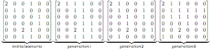
This is an example of 3 generations

You have to write a MATLB function that takes as input
• a 2D array that represents the initial scenario
• the number of generations and returns as output the evolved grid and the number of preys and predators alive at the end of the evolution process. The function, will implement the evolution of the system given the initial state and the number of generations.

At the beginning of your function you have to insert a check on the correctness of your inputs, namely
• the input 2D array needs to be square
• the input 2D array needs to be initialised with values 0-1-2, no other value is allowed
• the input number of generations needs to be positive
If any of the checks fails the function returns an error message to screen and exits by return- ing as output a scenario without preys or predators (zeros 2-D array) with number of preys and predators equal to zero.

Validation

This is an example that you can use to validate if your function works, where M is the input grid, 15 and 30 the number of generations used, G the evolved system, n the final number of preys and m the final number of predators:
>> M

M=
2 0 0 1 0 0
0 1 1 0 0 0
0 0 0 0 1 0
0 0 0 0 1 0
0 0 2 1 0 0
0 0 1 1 0 0

>> [G,n,m] =preypredator(M, 15 ) G=

2 0 0 0 0 1
0 0 0 1 1 1
0 1 1 0 0 1
0 0 1 0 1 0
0 0 2 1 0 0
0 0 0 0 0 0
n= 10
m= 2

>> [G,n,m] =preypredator(M, 30 )

G=

0 0 0 1 0 0
0 0 0 1 0 0
0 0 0 1 0 0
0 0 0 0 0 0
0 0 0 0 0 0

n = 3 m= 0