Reference no: EM132813882

MAE 3403 Computer Methods in Analysis and Design - Oklahoma State University

You will be writing three different Python programs in three different files named hw5a.py, hw5b.py and hw5c.py. You will place your files in a folder named HW5 and then zip the folder and upload it to Canvas.

In this assignment, you must use variables, loops, if statements, your own function definitions and function calls. For now, you may not use any of the powerful functions available in python modules, with a few exceptions: You may import functions from the math, copy, matplotlib.plot, numpyand scipy.

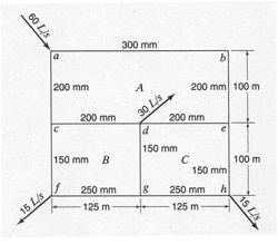
a.) A pipe network problem: Write a program that uses FSOLVE() to find the volumetric flow rate (m³/s) of water in each segment of the pipe flow network given below.

Use the following properties:
waterdensity = 1000 kg/m³
waterviscosity = 0.00089 N⋅s/m²
pipe roughness = 0.00025 m.

Your program should print the flow in each segment of pipe, nicely formatted, similar to:
The flow in segment a-b is -0.0052 m³/s
The flow in segment a-c is 0.0272 m³/s
The flow in segment d-g is -0.0142 m³/s
etc.
Notes:
Pressure decreases in direction of flow (e.g.,ΔP_(a→b)={(<0 if flow a→b

                                                                            {>0 if flow b→a))

The head loss around a pipe loop is zero. (e.g.,ΔP_(a→b)+ΔP_(b→e)-ΔP_(d→e)-ΔP_(c→d)-ΔP_(a→c)=0)
Mass is conserved at each node. ∑_i(m_i) ? =0
Pressure loss in a pipe is calculated with the Darcy-Weisbach equation: Δp=f L/D (ρV²)/2
Darcy friction factor is calculated by the Colebrook equation: 1/√f=-2.0log((e\/D)/3.7+2.51/(Re√f))

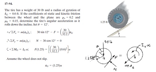
b. Write a program that uses FSOLVE() to solve the Rolling Wheel Dynamics - impending slip problem shown. You MUST use the "args" feature of Fsolve to communicate the wheel parameters. Use all of the wheel parameters posted, except for the static coefficient of friction and the ramp-angle θ. Generate a plot of ramp-angle vs coefficient of friction for impending slip, for friction values of 0.1, 0.15, 0.2, 0.25, up to 0.85.

c) The following differential equations describe the behavior of a hydraulic valve system

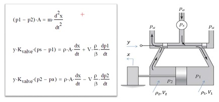
The values for the constant parameters are:

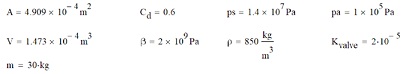
NOTE: All units for the variables and the constants are consistent as given, and no unit conversions of any kind are necessary.

Required:
Use odeint() to solve the differential equations for the response to a constant input of y=0.002

The initial conditions are: x=0, x?=0, p1=pa, p2=pa

1. From that solution, plot x? as a function of time, with nice title and labels.
2. From that solution, plot p1 and p2 together as functions of time, on a new graph, with nice title and labels and legend.

Attachment:- Computer Methods in Analysis and Design.zip