Reference no: EM133321219

Assignment: In this assignment you will practice Riemann and Stieltjes integration of non-smooth functions. You should be prepared that this assignment is the most challenging so far in the course and will most likely require substantial thinking.

Question 1. Integration: We introduce a sequence of continuous functions, f_j: [0, 1] → R,J = 1,2, 3,..... that converges to a function, f. In financial applications, these types of functions are usually defined over time so we will use t as the domain variable.

For J = 1, define

f₁(t) = t

Also, let us associate with f₁, the "dyadic" points t₀ = 0, t₁ = 1/2, t₂ = 1, the set X¹ = {t₀, t₁, t₂} and the partition of the interval [0, 1), into [t₀, t₁) and [t₁, t₂). Note that f₁ is a linear function on each of the subintervals in the partition (being a linear function on the whole of [0, 1]). More generally, for J ≥ 1, we define N = 2^J, the set X^J = (t₀, t₁...... t_N} = {0, 2^-J, 2x2^-J, 3 x 2^-J, ....1}, and the partition of the interval into subintervals, p^J = {[t₀, [t_1, t2 ),.......[t_N-1, t_N)}. The set of dyadic points is X^J = U_j=1^∞ X^J, which is obviously dense in [0, 1].

We will now use a clever approach to define the function f_j+1 from f_j in a way such that

• f_j+1(t) = f_J(t) for all t ∈ X^j, that is, the value of fj'(t) never changes in the dyadic points t ∈ C^J, as J' grows.
• fj is continuous for all j and linear on each of the subintervals in P^j.
• fj converges uniformly to a continuous function f:[0, 1] → R as J tends to infinity.

We proceed as follows: To define f₂, we keep the values f₂ (t) = f₁(t) at the points t ∈ X¹ = {0,1/2,1}. but we modify the values in X²\X¹ = {1/4, 3/4}, so that

f₂(1/4) = f1(1/4) - 1/√8 = (f₁(0) + f₁(1/2))/2 - 1/√8 = 1/4 - 1/√8 ≈ - 0.1036,

and

f₂(3/4) = f1(3/4) + 1/√8 = (f₁(1/2) + f₁(1))/2 + 1/√8 = 3/4 + 1/√8 ≈ 1.1036,

Thus, f2 is now defined for all elements of X². To extend f₂ to the whole of [0, 1], we simply make it linear on each of the intervals in p² = ([0, 0.25), [0.25, O.5) [0.75, 1)}, so that it is continuous on the whole of [0, 1], i.e., we "connect the end-points with straight lines."

We repeat this procedure to define functions fj : [0, 1] → R for J > 2. Specifically, given the continuous function f_j that is piecewise linear on each interval in p^j (and therefore completely defined by its values in X^J), we first define f_j+i(t) = fj(t) for all t∈X^J.

For t = (2k - 1)2^-(J+1) ∈ X^J+1\ X^J, k = 1,....2^J, we moreover define f_J+1(t) = f_J(t) + (-1)^k+j+1 2^-J/2-1, Finally, we extend the definition of f_j+1 from X^j+1 to the whole of [0,1], by "connecting the end-points with straight lines," thus making it continuous and piecewise linear. The functions f₁, f₂, f_3, f₄ are shown in Figure 1, below, and in Figure 2 the procedure has been further repeated for J = 4,....12.

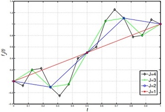
Figure 1: Functions f1, f2, f3, and f4.

You should take some time to make yourself comfortable with the properties cif these functions and the methodology used to construct them, Specifically, convince yourself that each function is continuous and piecewise linear on X^J, and that f_j(t) = fj'(t) for all t∈X^J and j' > j. Furthermore, note from Figure 2 that as J, grows, f_j converges to a function f that "wiggles" a lot but looks like it is continuous.

We analyze the smoothness properties of f. 'We begin by showing convergence of f_J to f. Recall that the space of continuous functions from [0, 1] to R, C([0, 1], R), is a Banach space under the sup-norm

||f|| = sup_{t∈[0, 1]}|f(t)|

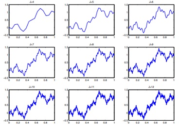
Figure 2 Functions fJ, J = 4,... , 12.

Such convergence is also called uniform {see lecture), and the norm is consequently called the norm of uniform convergence.

(a) Prove that the sequence f₁, f₂, converges uniformly to a continuous function, f: [0, 1] →R, by showing that it is a Cauchy sequence in the sup-norm.

Hint; In proving (a), it may be useful to use the fact that if {x_n} is a sequence in a normed space such that for some constants c > 0 and 0 < q < 1, and n > 1,

||x_n - x_n-1||≤ cqⁿ

then {x_n} is a Cauchy sequence. This follows from the fact that

x_m - x_n = (x_m - x_m-1) + (x_m-1 - x_m-2)+ .....+ (x_n+1 - x_n)

and therefore by the triangle inequality

||x_m - x_n|| ≤ ∑_{j= n+1}^m||x_j - x_j-1||≤c ∑_{k= n+1}^mq^-k = cqⁿ⁺¹ ∑_k=0 ^m-n-1  q^-k ≤ c(qⁿ⁺¹/1-q)

which tends to zero for Large n, so the condition. for being a Cauchy sequence is indeed satisfied. Here, we used the geometric summation formula to get the last inequality.

The limit function is thus continuous., but as mentioned it "wigglas' a lot, so we do not expect. it to be differentiable everywhere. In fact, it is far from differentiable as shown by our next result.

First, recall the definition of Holder continuity: f∈C^α([0, 1], R) if

sup_t,s≠t |f(t) - f(s)|/|t-s| < ∞, for some constant 0 < α ≤ 1.

As discussed in class, the higher α is, the smoother is f. For a function to be differentiable at a point, it must be locally Holder continuous of degree α = 1 at that point, since it must be that

|f(t) - f(s)|/|t-s|¹ ≈ |f'(t)|,

for s close to t or otherwise the derivative is not defined. Thus, at points where f ∈ C^α([(0, 1),R) for some α < 1, f is not differentiable.

(b) Consider an arbitrary dyadic point, t = k2^-j for some J > 0 and 0 ≤ k < 2^j. Show that for any such point,

|f_j'(t +2^-j') - fj'(t)| ≥ 2^-j'/2/8 for some J^' ∈ {J +1, J + 2}.

(c) Use your result in (b) to show that f ∈/ C^α([0, 1], R) for any dyadic t, for any α > 1/2.

The result in (c) is easily extended to hold for any (non-dyadic) point t ∈ [0, 1], and it thus follows that f is not differentiable anywhere. It can also be shown that f ∈ C^α([0, 1], R) for any α < 1/2 (you may wish to show this for dyadic points as extra practice), so in some sense f is "one half times differentiable" (the argument can be made exact but is outside of the scope of this assignment).

We next study integrals of f. First, note that since f is continuous (as shown in (a)), it follows immediately that it is Riemann integrable, i.e., ₀∫¹f(t).dt exists.

(d) Show that fj(t) = 1 - fj(1 - t] for all J and t, and use this result to show that ₀∫¹f_J(t).dt = 1/2 for all J ≥ 1 for all J > 1.

(e) Use your result in (d) to show that ₀∫¹f(t)dt = 1/2.

Although f's nonsmoothness is not an issue for Riemann integration, it is for the Stieltjes integral. We shall now show that the Stieltjes integral ₀∫¹f(t) df is not defined for this function. First, recall that Young's (1936) result implies that if f ∈ C^α for α > 1/2 then the integral ∫f.df is defined (see the class discuasion). Now, since f's Holder regularity in this case is just short of Young's result cannot he applied. Moreover_ note that under the even stronger condition of f being continuously differentiable, we would have ₀∫¹f(t) df = [f(t)²/2]₀¹ = (f(1)²- f(0)²/2) =1-0/2 = 1/2

For the Stieltjas integral ∫ f df to be defined, it must be that for any sequence of finer and finer partitions of [0,1], the upper and lower sums converge to the same number. Now consider the two sums

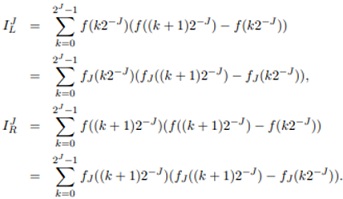
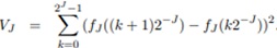
A necessary condition for the Stieltjes integral ∫f df to exist is then that lim_j→∞ I_L^J = lim_j→∞ I^J_R, since the I^J_L corresponds to a Riemann-Stieltjes sum over the partition X^J when the left end-point of each interval is chosen to evaluate f, and I^J_R is the sum when the right end-point of each interval is chosen. Equivalently, defining V_J = I^J_R - I^J_L the condition is that

lim_j→∞ V_J = 0

From (1) and (2) it follows that

(f) For t = k2^-j 0 ≤  k < 2^J, assume that f_j(t) = α and f_j (t) (t +2^-j) = b. It follows that (fj(t +2^-j) - fj(t))² = (b - a)². Show that

(f_(j+1)(t+2^-j-1)- f_j+1(t)² + (f_j+1 (t + 2^-j) - f_j+1 (t +2^-J-1))² = (b-a)²/2 + 2^-j-1.

(g) Use the result in (f) to show that V_J+1 = V_J/2 + 1/2 for all J ≥ 1, and that it therefore follows that

V_J = 1-2^-j

So. from (g) it follows that the Riemann-Stieltjes integral is not defined for f! In fact, one can show that lim_j→∞I^J_L = 0 and lim_j→∞I^J_R = 1. An intuition for why the sum is higher when the right end-point is used to evaluate f is as follows: When F((k + 1)2^-J) > f(k2^-J), df is positive, and should be multiplied by as large a number as positive to increase the sum in the integral. ie, by the right end-point. Similarly. when f((k +1)2^-J < f(k2^-J.) df is negative and a small number should be used to make the sum large. Again, the right-endpoint achieves this objective. To make the sum as small as possible, the left end point should then be chosen, and the difference between the sums that use the right and left endpoints will then be positive.

The above argument for how to make ∫g dg large also holds when g is a smooth differentiable function, but when the partition becomes fine enough in this case, the difference between using the left and right end-points in the sum becomes marginal for fine partitions, which is why the Stieltjes integral exists when g is smooth. Specifically, since |g(t + Δt) - g(t) ≤ C |Δt| for a smooth function, g, it follows that each term (g_j((k+1)2^-j) -g_J (k2-^J))² ≤  C2^-2J, and since there are 2^j such terms to be summed up, their sum is bounded by C2^-2j2^J = C2^-J, which in turn converges to zero for large J. For f on the other hand, |f (t + Δt) - f(t)| ~ C√Δt, and thus (f_J((k +1)2^-J) - fj(k2^-J))² ~ C2^-J. Summing up 2^J such square terms thus leads to l^J_R - l^J_L not decreasing to zero as J grows, as you proved in (f).

The reason we have spent such substantial effort on the exotic function f is that this function gets to the core of why Ito calculus is needed in continuous time finance. Specifically, the so-called diffusion processes that are extensively used in continuous time finance have very similar regularity properties as f As a consequence, they are not Riemann-Stieltjes integrable, but if the left end-point is consistently used in the summation-as done when calculating ill-the limit of the sums is defined. As will be discussed, it is the natural to use the left endpoint when defining integration in the context of stochastic integration, which leads to the Ito integral and in turn, to Ito's lemma and stochastic calculus!

Question 2. Finite difference method for Black shales PDE (in reflected log ca mites): Consider the double knock-out power option discussed in class. The underlying stock. price at time t is S_t. The initial stock price is S₀ ∈ (50,100), and the option's maturity date is T = 1, measured in years. The risk-free rate is r = 0.05 per year, and the stock's volatility is σ = 0.4 per year.

At expiration, if the stock price lies in the interval S ∈ (50,100), and its price has never been outside of this interval between 2 = 0 and T the option pays out:

P(S, T) = (5 - 50)(100 - S).

If the stock price has been outside of the interval, the payout is P(S, T) 0, i.e., the option is worthless. Since the price path of the stock is continuous (almost surely), this occurs if min_0≤t≤T S_t > 50 and max_0≤t≤T St < 100.

(a) PDE: Write the PDE for the price of this option, V(s,x), including boundary and initial conditions, in log space coordinates, x = ln(S), and reflected time coordinates, s = T-t.

(b) Solver: Implement a finite difference solver for the PDE, using the finite difference method with operators D₊₈, D_0x, and D_+xD_-x, for the different derivative estimates, as discussed in class.

You may use your favorite programming language (Matlab, Python, etc.), or even Excel. Please include your source code (or in case of Excel, your spreadsheet) with your submission.

(c) Solution; Using the ratio between time and space step-length k = Δt/Δx² = 2, calculate the approximate solution at t = 0, with Δx = 100 points.

• Please include graphs of V(x, 0), V(x, 1), P(S 1) , and P(S, 0).
• Where does the value (in S coordinates) reach its maximum?
• The maximum value of the payouts P(S, T) is reached at S = 75. Why do you think the maximum value of P(S, 0) is reached at a different value of S?
(d) Stability: Vary k. How large can k be while keeping the approximation method stable? Does this bound on k depend on ΔX?
(e) Order of convergence: Vary Δx, keeping k =1/4 constant. Estimate the order of convergence of the approximation method to the true solution.

Question 3. Black scholes PDE: In a market in which the Black Scholes assumptions are satisfied, an asset makes the terminal payoff

f(S(T)) = S(T)ⁿ, n > 1

where S(T) is the value of the underlying stock at time T. The asset's value if the stock price reaches zero is P(0, t) = 0,

(a) Show that the price of this power asset at 0 < t ≤ T is

P((S(t), t) = e^{((n- 1)r+n(n-1)σ2/2)(T-t)}S(t)ⁿ.

Question 4. Ito's lemma; Consider the stochastic process

dX_t = μdt + σdW_t

Find a closed form expression for Q, defined by the stochastic integral

Q = ₀∫^T 3x_t(μXt + σ²)dt + 3X_t²σdW_t,

by postulating a function G(t, W_t) that satisfies dG_t = 3X_t(μX_t + σ²)dt + 3X_t²σd.W_t, and using the definition of the stochastic integral in class to get Q = G(T, W_T) - G(0, W₀).

Question 5. Optimal control: Consider an investor with utility function

U = ∑_t=0^T ρ^t ln(c_t), 0 < ρ < 1

As in class, each period the investor chooses consumption c and investment I_t = W_t - c_t. Investments grow at the stochastic rate R_t between t and t +1, where R_t depends on the value of s_t+1, which follows an N-state Markov process with transition matrix Φ ∈ R₊^NxN. As
in class, returns are summarized by the N-vector R ∈ R₊₊^N. The agent faces the constraint that W_t ≥ 0 at each point in time.

(a) Find the optimal consumption policy, c(t, W_t) and indirect utility function J(t, W_t), for all t ∈ {0,1......,T}

(b) How does the consumption policy depend on investment returns, R? Discuss whether the formula is reasonable.

(c) Calculate the optimal consumption policy and indirect utility function in the infinite horizon case, i.e.. in the limit when T →∞.

Question 6 Probability spaces: Consider the state space Ω = {ω₁, ω_2, ω_3, ω₄} with associated σ-algebra F = 2^Ω and probability measures, P, and Q, defined by:

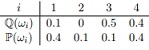
(a) Are P and Q equivalent probability measures?

(b) What is the Radon-Nikodym derivative, L = dQ/dP?

Question 7: Meastrability: Consider the state space Ω = R, the σ-algebra, F = {(-∞, 0],  (0, ∞),ø, R} and the random variable X : Ω → R defined by

X(ω) = 3, ω < 0,

X(ω) = 5, ω ≥ 0,

Is X F-measurable?