Reference no: EM13381210

Part 1 - Generating Random Variables

Most software libraries include a uniform random number generator that generates equally probable numbers between 0 and 1. A uniform RV can be used to generate random variables with other distributions. For example suppose that we want to generate a new random variable X with pdf f_X. Specifically, we want to generate a Gaussian random variable with the following pdf:

where σ_x²  is the variance of the distribution and μ_x is the mean.  

We also know that the probability

is a number between [0,1], that we will denote as "A". If we want to find out what value of x0 will make the integral in (2) equal to A, an inverse mapping for the integral in (2) needs to be evaluated. Unfortunately it is hard to express the integral in (2) in terms of simple functions.

In EE-131A & B, we also learned about the relationship between Rayleigh and Gaussian distributions. The Rayleigh CDF can be expressed as

where r is related to a pair of Gaussian random variables by the transformation

and σ² is the variance of both the Gaussian RVs.

The function in (3) is a lot simpler to invert than the integral in (2):

We can also generate a second uniformly distributed random variable B~U[0,1]  and define θ = 2ΠB.

Your  task: Write the proper code such that:

• Complete the missing portion of the a function GenerateGauss(mu,sigma²) that will generate a two Gaussian random variables from a single uniform random variable u.
  • If the function is given no arguments, then the default settings are mu=0, sigma²=1
  • If only one argument is given then we assume that value is the variance, and assume mu=0
• You will see that the function you wrote is much slower than the internal Matlab function. To make the code a bit more efficient, generate a new function GenerateGaussVector(mu,sigma²,N).
  • You should expect to be much faster than the original one you wrote, however you probably won't be able to beat Matlab's internal function randn.(Matlab's internal function is probably around 4 times faster than your version of GenerateGaussVector )
  • For this section your code has 3 inputs. If less than 3 inputs are given by the user then you should do the following. If GenerateGaussVector(arg1, arg2, arg3).

- 0 args: Generate TWO random variables with distribution Gaussian(0,1)  

- 1 arg: Generate TWO random variables with distribution Gaussian(arg1,1)

- 2 args: Generate TWO random variables with distribution Gaussian(arg1,arg2) 

- 3 args: Generate a vector (of even length) with random variables of dimension N=arg3 with distribution Gaussian(arg1,arg2). For example:

• GenerateGaussVector(a, b, 4)-> Generates 4 RVs with dist. Gaussian(a,b)
• GenerateGaussVector(a, b, 5)-> Generates 4 RVs with dist. Gaussian(a,b)
• GenerateGaussVector(a, b, 6)-> Generates 6 RVs with dist. Gaussian(a,b)
  • For this section, you do not need to handle the special case where the input is GenerateGaussVector(a, b, 1)
• GenerateGaussVector(arg1, arg2, 1)à Generates an empty vector
• Again, for this section you do not need to worry about the special case of N=1 for the problems on this section

When you open the provided Matlab files, you will see sections labeled like this:

You are only supposed to modify the portion of the code marked.

The way it's written, the "skeleton" code provided will run. However, the outputs will likely be all zeros.

When a vector of zeros is defined between the lines of code that you are supposed to edit, be smart to realize that your solution should have the same dimensions as the vector you are replacing

Once you are done writing your functions, your output should look somewhat like this (the numbers may vary a bit ...)

Matlab Function: Mean=9.9984  Var=3.9750
EE131B Function: Mean=10.0055 Var=4.0024

Matlab Internal Function is 87.03 times faster than ours
Matlab Internal Function is 1.76 times faster than our vector function
The vector function is 49.58 times faster than our 1-D function

Part 2 - Generating Multivariate Random Variables

For our next application, we want to generate a multivariate Gaussian random variable.  Your function will now take as inputs

• A vector of mean values: mx
• A covariance matrix: Cx

And will use your function GenerateGauss to compute the two dimensional pdf.

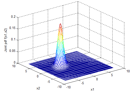
In part (c) you will do a 3-D plot of the multidimensional Gaussian pdf, according to:

Complete the code in the Matlab script "ProjectPart_02.m"  to compute the two dimensional pdf.

Use the "mesh" function in Matlab to display your result

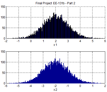
Your output should look like this

My Vector of Means values is mx=[2.0, -2.0]
My autocorrelation matrix is Cx=
[     1.00 0.50 ]
[     0.50 1.00 ]

The Dimensions of my vector of Gaussian RVs is [2 x 1]
The mean and variance of my 2-D Gaussian Vector are:

      Mean=[2.01 , -1.99] 
      Var =[1.01 , 1.01]

Hints:

In Matlab, the function sqrtm() can be used to take the square root of the autocorrelation matrix. You may choose to use this function when you write the code for multidimensional_gp to properly scale the output vector

Cx =
    1.0000    0.5000
    0.5000    1.0000

>>  X = sqrtm(Cx)

X =
    0.9659    0.2588
    0.2588    0.9659

Part 3 - Power Spectrum of a Random Process

A random process X(t) can be characterized in the frequency domain by its power spectral density S_XX(f), which is the Fourier transform of the autocorrelation function R_XX(τ)

Your Task:

Complete the code in "ProjectPart_03.m". This involves:

• Generating a discrete time sequence of IID uniformly and Gaussian distributed random numbers
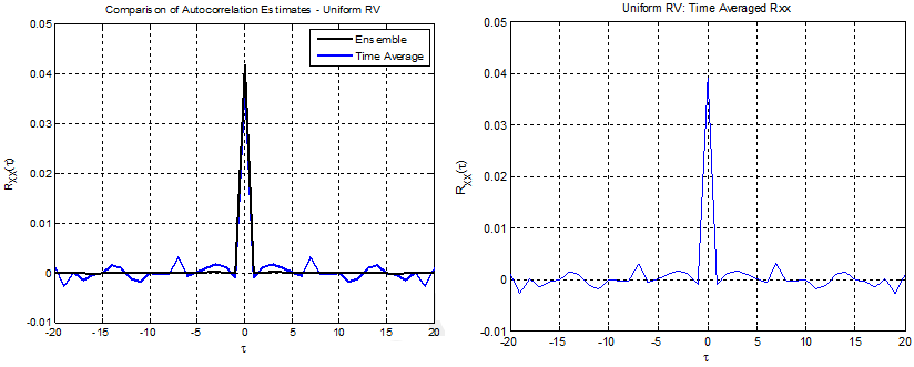
• Computing the estimate of the autocorrelation of the sequence {X_n} by doing an ensemble average

Note: In the equation above you can  the Matlab functions conv or xcorr to compute the integral or you can write your own function to perform the integration. In order to obtain the right result, make sure to properly normalize by the vector t.

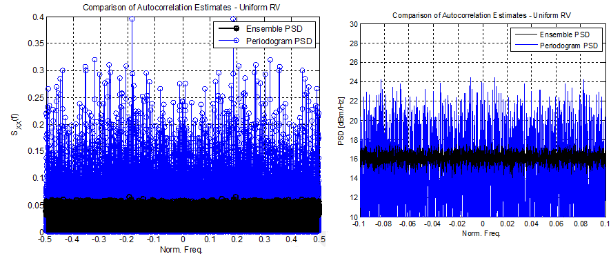
• Computing the PSD of the sequence {X_n} using the periodogram method and a single realization of the random sequence {X_n}

• Comparing the performance of an ensemble average vs. a single realization average

Tasks:

a) Run the Code using the variable

MyDistribution =1; % Uniform Random Variable

Your output should look like this

Project - Part 3
Uniform RV
Ensemble    PSD: Mean=0.044
Periodogram PSD: Mean=0.039

And the following 4 figures should be generated

b) Run the Code using the variable 

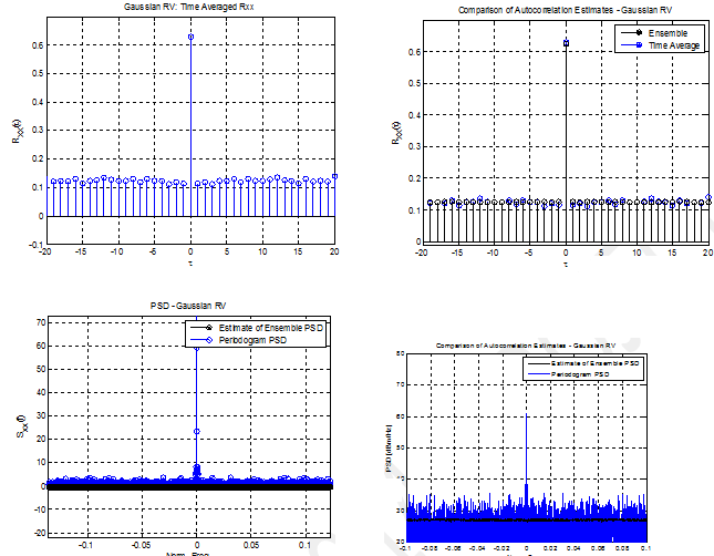
MyDistribution =2;    % Gaussian Random Variable

 Your output should look like this

Project - Part 3

Gaussian RV

Ensemble    PSD: Mean=0.672

Periodogram PSD: Mean=0.563

And the following 4 figures should be generated

Download:- Project.rar