Reference no: EM132590124

EE-524 Assignment - Assume the valid values for the parameters wherever it is necessary.

Q1. Consider the following transfer-function system:

Y(s)/U(s) = s + 6/s² + 5s+ 6.

Obtain the state-space representation of this system in (a) controllable canonical form and (b) observable canonical form.

Q2. Consider the following system:

y^··· + 6y^·· + 11y^· + 6y= 0.

Obtain a state-space representation of this system in a diagonal canonical form.

Q3. Consider the system defined by

x^· = Ax + Bu

y = Cx

where

Obtain the transfer function Y(s)/U(s).

Q4. Consider the following matrix A:

Compute the e^At by two methods.

Q5. Find x₁(t) and x₂(t) of a system which is described by

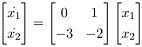
Assume any initial value you like.

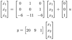
Q6. Consider the system given by

Is the system completely state controllable and completely observable? Determine controllability and observability Gramian.

Q7. Is the following system completely state controllable and completely observable?

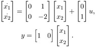
Q8. Obtain the discrete-time state and output equations (when the sampling period T=1) of the following continuous-time system:

Q9. Obtain a state-space representation of the system described by the equation:

y(k+ 2) + y(k+ 1) + 0.16y(k) = u(k+ 1) + 2u(k)

Comment on stability.

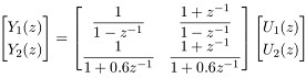
Q10. Obtain a state-space representation for the system defined by the following pulse-transfer-function matrix:

Q11. Consider the discrete-time state equation

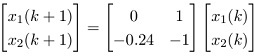
Obtain the state transition matrix ψ(k).

Q12. Consider the system defined by

x(k+ 1) = Gx(k) + Hu(k).

Solve x(k) for an initial value x(0) = x₀.

Q13. Consider a system defined by the equations

x₁(k + 1) = x₁(k) + 0.2x₂(k) + 0.4

x₂(k + 1) = 0.5x₁(k) - 0.5,

determine the stability of the system.

Q14. A non-linear system is given as x^· = 4x³ + 3 with x(0) = 3. Linearize the model about the origin. Solve the state equation for the linearized system. Solve the non-linear model for the state using Runge-Kutta method. Plot the two solutions and comment.

Q15. Consider the following model for a two-phase permanent magnet synchronous motor:

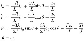
where i_a and i_b are the currents through the two windings, R and L are the resistance and inductance of the windings, θ and ω are the angular position and velocity of the rotor, λ is the flux constant of the motor, u_a and u_b are the voltage applied across the two windings, J is the moments of inertia of the rotor and its load, F is the viscous friction of the rotor, and T_l is the load torque.

Find out the Jacobians w.r.t. the state vector(x= [i_a i_b ω θ]^T) and the input control vector [u_a, u_b]^T. Linearize the non-linear model around a general nominal value x^- and u^-. Simulate the non-linear and the linearized model (Suggestion: a nominal control input [u^-_a u^-_b]^T = [sin 2πt cos 2πt]^T and the resulted state trajectory x^-(t) can be used for the simulations). Plot (using MATLAB/C) the different states of the two models.