Reference no: EM131858750

MATLAB solvers for First-Order IVP

In this laboratory session we will learn how to

1. Use MATLAB solvers for solving scalar IVP

2. Use MATLAB solvers for solving higher order ODEs and systems of ODES.

EXERCISES

Instructions: For your lab write-up follow the instructions of LAB 1.

1. (a) Modify the function ex_with_2eqs to solve the IVP (L4.4) for 0 ≤ t ≤ 50 using the MATLAB routine ode45. Call the new function LAB04ex1.

Let [t,Y] (note the upper case Y) be the output of ode45 and y and v the unknown functions. Use the following commands to define the ODE:
function dYdt= f(t,Y) y=Y(1); v=Y(2);
dYdt = [v; sin(t)-7*v-5*y];

Plot y(t) and v(t) in the same window (do not use subplot), and the phase plot showing v vs y in a separate window.

Add a legend to the first plot. (Note: to display v(t) = yj(t), use 'v(t)=y''(t)').

Add a grid. Use the command ylim([-1.2,1.2]) to adjust the y-limits for both plots. Adjust the x-limits in the phase plot so as to reproduce the pictures in Figure L4g.

Include the M-file in your report.

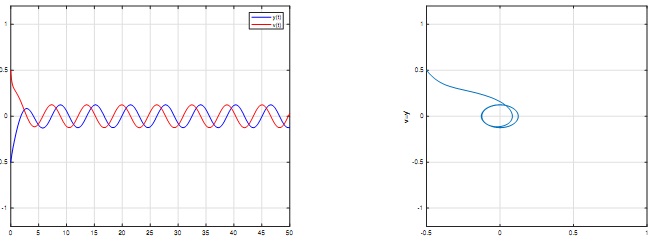
Figure L4g: Time series y = y(t) and v = v(t) = y'(t) (left), and phase plot v = y' vs. y for (L4.7).

(b) For what (approximate) value(s) of t does y reach a local maximum in the window 0 ≤ t ≤ 50? Check by reading the matrix Y and the vector t. Note that, because the M-file LAB04ex1.m is a function file, all the variables are local and thus not available on the Command Window.

To read the matrix Y and the vector t, you need to modify the M-file by adding the line [t Y].
Do not include the whole output in your lab write-up. Include only the values necessary to answer the question.

(c) What seems to be the long term behavior of y?

(d) Modify the initial conditions to y(0) = 2, v(0) = 3 and run the file LAB04ex1.m with the modified initial conditions. Based on the new graphs, determine whether the long term behavior of the solution changes. Explain. Include the pictures with the modified initial conditions to support your answer.

EXERCISES

2. (a) Consider the modified problem

d²y/dt² + 7y².dy/dt + 5y = sint, with y(0) = -0.5, dy/dt(0) = 0.5

The ODE (L4.7) is very similar to (L4.4) except for the y² term in the left-hand side. Because of the factor y² the ODE (L4.7) is nonlinear, while (L4.4) is linear. There is however very little to change in the implementation of (L4.4) to solve (L4.7). In fact, the only thing that needs to be modified is the ODE definition.

Modify the function defining the ODE in LAB04ex1.m. Call the revised file LAB04ex2.m. The new function M-file should reproduce the pictures in Fig L4h.

Include in your report the changes you made to LAB04ex1.m to obtain LAB04ex2.m.

(b) Compare the output of Figs L4g and L4h. Describe the changes in the behavior of the solution in the short term.

(c) Compare the long term behavior of both problems (L4.4) and (L4.7), in particular the am- plitude of oscillations.

(d) Modify LAB04ex2.m so that it solves (L4.7) using Euler's method with N = 1000 in the interval 0 ≤ t ≤ 50 (use the file euler.m from LAB 3 to implement Euler's method; do not delete the lines that implement ode45). Let [te,Ye] be the output of euler, and note that Ye is a matrix with two columns from which the Euler's approximation to y(t) must be extracted. Plot the approximation to the solution y(t) computed by ode45 (in black) and the approximation computed by euler (in red) in the same window (you do not need to plot v(t) nor the phase plot). Are the solutions identical? Comment. What happens if we increase the value of N ?

Include the modified M-file in your report.

3. Solve numerically the IVP

d²y/dt² + 7y.dy/dt + 5y = sint, with y(0) = -0.5, dy/dt(0) = 0.5

in the interval 0 ≤ t ≤ 50. Include the M-file in your report.

Is the behavior of the solution significantly different from that of the solution of (L4.7)? Is MATLAB giving any warning message? Comment.

4. (a) Write a function M-file that implements (L4.8) in the interval 0 ≤ t ≤ 50. Note that the initial condition must now be in the form [y0,v0,w0] and the matrix Y, output of ode45, has now three columns (from which y, v and w must be extracted). On the same figure, plot the three time series and, on a separate window, plot the phase plot using

figure(2); plot3(y,v,w,'k.-');

grid on; view([-40,60])
xlabel('y'); ylabel('v=y'''); zlabel('w=y''''');

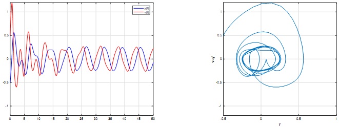
Figure L4i: Time series y = y(t), v = v(t) = y'(t), and w = w(t) = y'(t) (left), and 3D phase plot v = y' vs. y vs w = y'' for (L4.8) (rotated with view = [-40,60]).

Do not forget to modify the function defining the ODE.

The output is shown in Fig. L4i. The limits in the vertical axis of the plot on the left were deliberately set to the same ones as in Fig. L4h for comparison purposes using the MATLAB command ylim([-1.2,1.2]).

Include the M-file in you report.

(b) Compare the output of Figs L4h and L4i. What do you notice?

(c) Differentiate the ODE in (L4.7) and compare to the ODE in (L4.8).

(d) Explain why the solution of (L4.7) also satisfies the initial conditions in (L4.8). Hint: Sub- stitute t = 0 into (L4.7) and use the initial conditions for y and v.